Performance Engineering

October 2020: What makes supercomputers special? They have state-of-the-art processors, fast parallel file systems, specialized power & cooling infrastructure and complex software stack to run. But, a high-speed interconnect that tightly integrates thousands of nodes differentiate a supercomputer from a commodity cluster. Data movement within a node or across nodes is an important aspect for many scientific applications and hence low latency, high bandwidth interconnect technology is one of the key elements of the HPC systems.

Setting up such a system with tens of thousands of nodes and performance tuning is not an easy task. Especially during the early days of deployment and acceptance benchmarking where we often have to run various tests for weeks to identify issues, fix them and reach expected performance. Also, during normal operation of the system we have to make sure that software or hardware upgrades don't result in performance degradation. As network fabric being the key element, the network needs to be in healthy state. This often involves making sure the latency is the lowest possible and bandwidth is the highest possible across all compute nodes.

For measuring communication performance we often use benchmarks like OSU Micro-Benchmark (OMB) and Intel MPI Benchmark (IMB). These benchmarks are good at measuring performance using low level communication primitives. For example, OMB's point-to-point benchmark (osu_latency or osu_latency_mp) is used to measure latency between two nodes. But, if we need to test thousand of nodes and check if the connection between every node pair has expected performance then this becomes quite cumbersome. The Intel MPI Benchmark provides parallel PingPong and it can be run on multiple pairs simultaneously and measure average latency and bandwidth. But, these micro benchmarks are not designed to debug performance issues at scale. For example, what if one of the links is faulty or some nodes are running slow which result into unexpectedly high latency for certain pairs or affecting collectives? How can we easily find such a faulty link or a bad node? There are some vendor specific low level performance measurement and diagnostics utilities (e.g. ib_read_bw, ib_read_lat) but they have similar limitations and don't help to reveal high level software stack issues (e.g. MPI). As system size increases, it becomes harder to do performance troubleshooting and that's where LinkTest comes handy!

The LinkTest tool is developed at Jülich Supercomputing Centre (JSC), Germany. It helps to measure latency and bandwidth between a large number of node pairs and identify communication issues. Even though the tool is somewhat old and not updated during the last few years (hope to have a new version soon!), what I found unique about the LinkTest is the ease of use and intuitive way to present communication metrics. The tool has been designed with the scalability in mind and has been used on systems like JUQUEEN with more than a million MPI tasks.

If you are a system engineer, performance analyst or application developer, I believe LinkTest is a good tool to have in your arsenal. So let's get started!

How LinkTest works? How can it help?

The LinkTest implements a well known PingPong benchmark which was first published as part of Pallas MPI Benchmark suite (now Intel MPI Benchmark). If we run LinkTest with N MPI ranks on M nodes then LinkTest internally executes N-1 steps where every rank communicates with all other N-1 ranks. In each step, N/2 pairs are formed and each pair performs PingPong benchmark simultaneously. After running all steps, LinkTest records a full communication matrix with message latency and bandwidth between each node pair. Different performance reports generated by LinkTest can help to:

• find out latency and bandwidth between different cores, sockets or node pairs
• identify slower communication links efficiently
• simulate communication pattern and find out the communication cost
• generate performance report to identify the communication cost patterns

With these features, LinkTest can be a valuable tool to identify communication bottlenecks, bad links or misconfiguration during system deployment or after hardware/software maintenance.

Structure of LinkTest Performance Reports

One of the important aspects to use any profiling tool effectively is to develop a good understanding of the performance report and metrics reported. So before looking at the actual reports, let's look at the structure of a typical report generated by the LinkTest and understand how to interpret it.

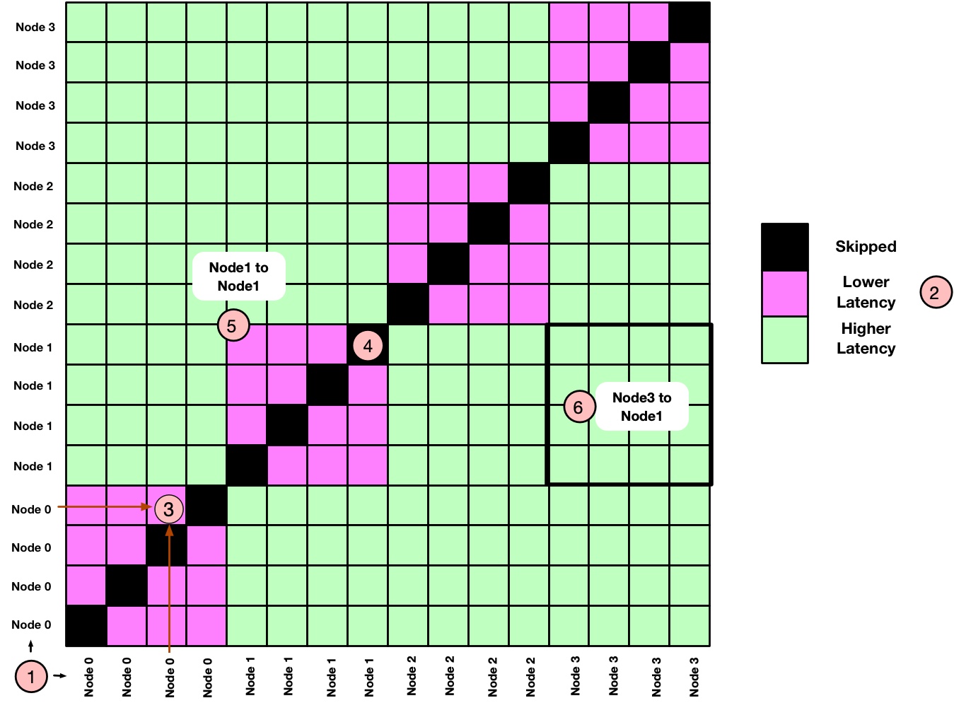
Let's assume we have a system with 4 nodes and each node has a single CPU with 4 physical cores. These nodes are named from Node 0 to Node 3. We are going to run a job with a single MPI task per core. If we run the LinkTest to generate latency communication matrix then the report should look something like below:

Let's try to understand this hypothetical report and highlight some important aspects:

• (1) shows the labels for the X and Y axis. As the plot represents the communication matrix between MPI ranks, both X and Y axis represent the MPI processes running on the corresponding nodes.
• If a node name is repeated N times then there are N MPI ranks running on that particular node. In our case we are running 4 MPI ranks per node.
• (2) shows the legend for latency or bandwidth. In the actual report this will be a color bar showing latency as well as bandwidth. For the simplicity we have shown just 3 colors.
• Each tile represents the PingPong latency (or bandwidth) between two ranks. For example, (3) shows the communication latency between 3rd and 4th ranks executing within Node 0.
• All diagonal tiles are black (4) because they represent PingPong tests with the same rank and LinkTest skip such tests.
• With N ranks executing per node, NxN tile represent the PingPong latency within a node or across nodes. For example, (5) shows intra-node latency between the ranks executing on Node 1 whereas (6) represents inter-node PingPong latency between ranks executing on Node 3 and Node 1.
• All 4x4 tiles showing intra-node communication (e.g. Node 0 to Node 0, Node 1 to Node 1) are shown with the same pink color. This means the PingPong latency between all four ranks is the same when they are communicating within the node. In practice there will be differences (e.g. due to system noise, NUMA etc). The same applies to inter-node communication where we have shown them with lime color.

Now let's assume a hypothetical scenario where we have one "bad node", for example Node 0 in this case. How do we expect the communication matrix to be affected? It's true that the effect of a "bad node" depends on various factors and type of issue (e.g. link is faulty, CPU is slow, orphan processes running etc). But assume a simple scenario where the issue is local to the node and not related to the network. In this case a simplistic view could look like the following:

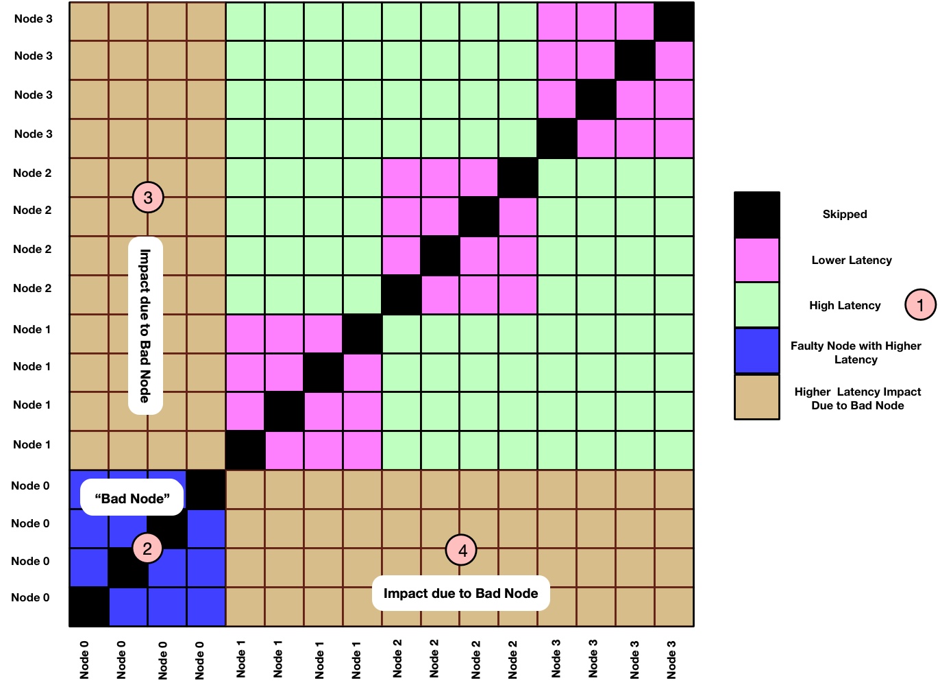
Based on previous discussion we can already guess what's going on. Here are some explanatory comments:

• As Node 0 is a "bad node" here, it is now shown with high PingPong latency (2). We expect its performance to be lower than other intra-node communications performance seen for Node 1, Node 2 and Node 3.
• Other nodes communicating with Node 0 will see impact on communication performance. This is shown by brown color in (3) and (4).
• As the issue is local to Node 0, we don't expect the impact on communication latency when Node 1, Node 2 and Node 3 are communicating within themselves. (this is a simplistic assumption.)

Obviously this is a hypothetical scenario and the real world picture will be different. For example, the communication cost will differ based on network topology, position of the nodes, network adapter placement on a NUMA node etc. But with the above discussion, you can already build a mental model of how latency distribution should look like on a given system.

We have now covered sufficient theoretical background. Let's now set up LinkTest and look at some real world performance reports.

STEP 0 : Installing LinkTest

Installing LinkTest is easy. It has dependency with MPI and SIONlib which is a scalable I/O library for task-local files. I have recently added LinkTest package to Spack. So if you are using Spack then you can install and use LinkTest as:

and we should be good to go! If you want to install via source tarballs instead, then it's also straightforward. First download tarballs as:

Assuming MPI compilers are available in $PATH, we can build LinkTest as:

Let's now add LinkTest installation directory to $PATH if you have installed from source tarballs:

With this we should have mpilinktest and pingponganalysis binaries available in $PATH. The mpilinktest is the main benchmark that runs PingPong test. The pingponganalysis is the analysis tool that reads performance data produced by mpilinktest and helps to generate various reports.

Here are some additional details for installation:

• SIONlib has options for choosing compiler suite (--compiler=), MPI library (--mpi=) etc. Check ./configure --help for details.
• LinkTest provides Makefiles for Linux and (old) BlueGene platforms. Makefile_LINUX is quite generic and can be modified to change compilers or platform specific flags.

Issue on macOS Using Preview

LinkTest generate performance reports in the PostScript format. If you are using macOS then  the Preview application doesn't interpret the reports generated by LinkTest version 1.2p1 correctly. It shows colors with the gradients and the report becomes difficult to understand. To workaround this issue we can convert postscript file to pdf (e.g. using ps2pdf ) and then use Adobe Reader or Chrome browser to view the generated pdf report.

STEP 1 : Running Latency Test Between A Node Pair

We are now ready to take the LinkTets for a ride. To begin with, we will use two compute nodes where each node has two Intel Cascade Lake CPUs (i.e. 2 sockets, each socket with 20 physical cores). For completeness, I have copied SLURM jobscript showing job parameters, benchmark options and commands used to generate performance report:

If you are running this test on your desktop then you can directly run commands shown above. Most of the jobscript is self-explanatory:

• We are submitting a SLURM job using 2 nodes with 40 MPI processes per node. Note that the LinkTest expects an even number of MPI processes.
• We run mpilinktest binary which is the main LinkTest benchmark. The CLI argument -s 1 indicates the message size of 1 byte for PingPong, -I 10 indicates warm up iterations and -i 10 indicates 10 iterations of the PingPong test.
• Once the mpilinktest finishes execution, it writes performance data in the SION file pingpong_results_bin.sion.
• We now use the pingponganalysis tool to analyse the performance data from the SION file and generate a postscript report.
• As mentioned in the installation section, the Preview application on macOS doesn't handle postscript report properly and hence we converted the report to pdf format using ps2pdf. Make sure to use Adobe Reader or Google Chrome to view the report on macOS.

Let's now look at the pdf report generated by pingponganalysis. Note that the labels are not clearly visible, but you can download the full PDF report from here. Also, we will not focus on the absolute performance numbers but relative performance as tests were performed on the test nodes of a busy system. Based on the discussion in the section Structure of LinkTest Performance Reports, we know how to interprete the report. Considering this test was performed on 2 nodes where each node has two Intel Xeon CPUs, can you analyze the report? Here are some explanatory notes to help:

• (1) on the right shows the color bar where lower latency values are at the top and higher latency values are at the bottom. It shows latency in usec (2) and corresponding bandwidth in MB/s (3).
• Four main quadrants (4), (5), (6) and (7) shows communication between node pairs. For example - (4) represents ranks on the Node 0 performing PingPong with other ranks on the same node; (5) represents ranks on the Node 1 performing PingPong with ranks on the Node 0.

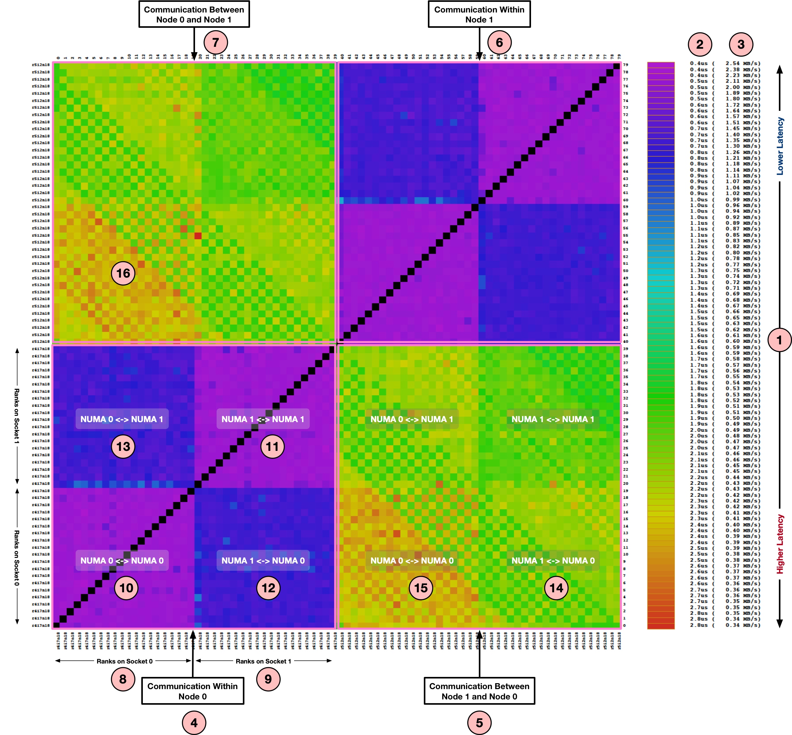
We can now focus on (4) which represent the intra-node communication for Node 0:

• As discussed earlier, the X and Y axis represents the ranks participating in the PingPong test. As this node has two sockets, (8) represent 20 ranks on the first socket whereas (9) represent next 20 ranks on the second socket. 
• (10) represent the communication matrix for ranks doing PingPong within Socket 0 of Node 0. As all communication remains within the same socket, the latency is lowest (~0.5 usec). Same is the case for (11) representing the Socket 1.
• (12) represent the communication matrix for ranks doing PingPong across sockets i.e. MPI ranks from the Socket 1 are communicating with the ranks on the Socket 0. As this requires communication across chips (e.g. over QPI), the latencies are higher than on-chip communication seen in (10) and (11). Same applies to (13) where ranks from the Socket 0 are communicating with the Socket 1.
• Similar to the quadrant (4), the quadrant (6) represents intra-node communication and shows almost identical communication latencies.

Let's now look at the quadrant (5) which shows an example of inter-node communication i.e. the ranks from the Node 1 are performing PingPong with the ranks on the Node 0.

• (14) represents the communication matrix for ranks on the Socket 1 of Node 1 communicating with the ranks on the Socket 0 of Node 0. As this  involves communication across the nodes, we see higher latencies (~2.0usec) than what we have seen until now.
• (15) represents the communication between ranks from Socket 0 of Node 1 with the ranks from the Socket 0 of Node 0. This is also inter-node communication like (14). But you might have already noticed higher latencies (~2.7us) than what we have seen in (14). Can you guess what could be the reason? If we look at the node topology using lstopo or ibdev2netdev then we can find out where the network adapter is connected:

As shown above, the network adapter is connected to the Socket 1 i.e. second numa node and hence the latency sensitive benchmarks like PingPong have higher latency when running on the Socket 0.

Let's now look at the second part of the report which contains a histogram and summary of the benchmark:

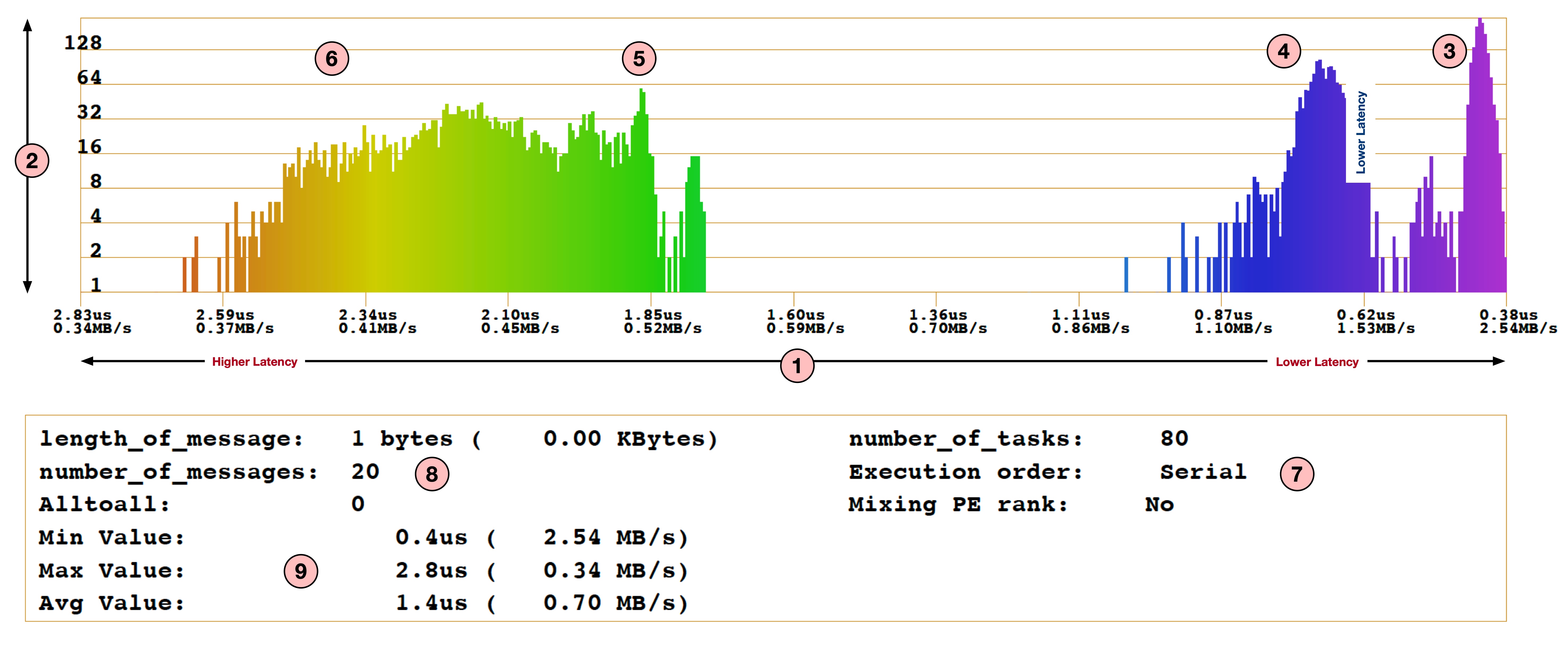
• For the histogram, X-axis shown by (1) is latency in usec (higher on the left and lower on the right) and the Y-axis (2) represents the number of messages with corresponding latency.
• With (3), (4), (5) and (6) we clearly see the distribution of latencies in four different groups: when ranks are communication within the same socket, when ranks are communicating within a node but across sockets, when ranks are communicating across nodes with Socket 1 and when ranks are communicating across nodes with Socket 0.
• (7) shows the number of MPI ranks used and indicates that this benchmark was run in Serial mode (see last section about Serial vs Parallel mode).
• (8) shows the message size used (1 byte in this case) and number of messages per test.
• (9) shows the minimum, maximum and average latencies achieved for this benchmark.

This histogram can be quite useful to get an insight into communication cost and system topology. 

STEP 3 : An Example of LinkTest At Scale

As mentioned in the introduction section, LinkTest is designed to be a scalable tool and can be run on hundreds of thousands of MPI processes. The report structure remains the same despite the number of MPI ranks. In this section we will look at one such example of the report with 28k MPI ranks. I haven't attached the pdf report as it was quite big (~100 MB).

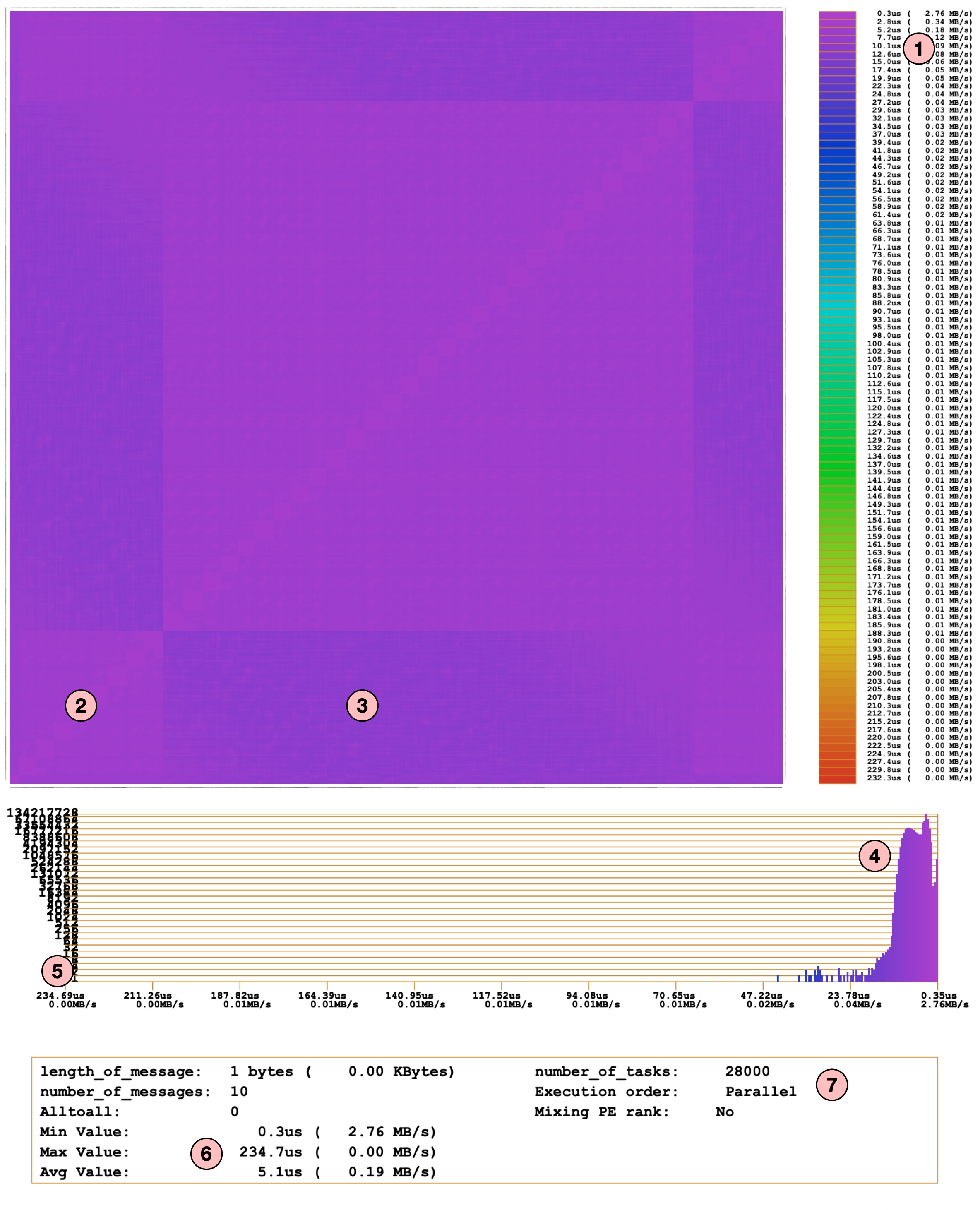
We will not dive into too many details as the report structure is similar to what we have seen before. Here is a short summary:

• (1) shows the latency and bandwidth color bar. Note that the X and Y axis labels for the heatmap are almost invisible because of the large number of data points (i.e. 28k ranks).
• (2) and (3) highlights small differences in the latencies. This indicates that there are certain nodes with higher latencies (around the borders). But if we look at the histogram (4), overall latency across the entire system is quite similar (~ ≤ 15usec).
• The highest latency observed was 234.7 us as shown in (6).
• If we look at the histogram (5), the total number of pairs with very high latency are very few (and hence the count is invisible on the histogram). This is a good news because communication performance looks consistent across the entire system.
• (7) shows the number of MPI ranks and the execution mode (parallel) used for this test.

This looks great! The LinkTest provides a great insight into overall system state and communication performance. But, you might be wondering about the highest latency (~234 usec) and how to dig into the details of a possible issue. By looking at the heatmap and histogram we can't find any insights. Let's see how LinkTest can help with this.

STEP 4: Understanding Performance Issues

One of the key feature of LinkTest is that it helps to find out the slowest link pairs effectively. In order to do this, LinkTest looks at the measured data and finds out the slowest pairs (e.g. with the highest latencies). It then re-run the PingPong across these slowest pairs to rule out any noise in the measurements. It then prints all pairs with the latencies measured during first as well as 2nd run. One can choose the number of the slowest links to find using the CLI option -Z.  Here is an example of one such run with 4 ranks. We chose a small number of ranks to minimize the output:

In the above example there are a total 3 steps executed. During every step the LinkTest shows min, max and avg latency measured for that particular step. After all steps are finished, it prints out the min, max and avg latencies across all steps. As we have provided -Z 2 CLI argument, the LinkTest searched for two slowest communication pairs and re-run the PingPong with those two pairs. The numbers printed after 2nd: indicates the latencies measured in the 2nd execution of the PingPong. If the performance is still low then one can perform other diagnostic tests on the corresponding node pair.

Using Serial Mode

The LinkTest also provides Serial mode to run PingPong (with CLI argument -S 1). In the serial mode only one pair of MPI ranks perform PingPong at a time. This is useful if we want to run PingPong without any interference from other ranks or avoid bandwidth saturations when using larger message sizes:

In the above execution we have used the -S 1 option to run the benchmark in serial mode. The output is the same as what we have seen before. The only difference is that the PingPong test is now performed with one pair at a time and corresponding latency numbers are printed. Note that this significantly increases the execution time. But it is useful if we want to focus on a small subset of tasks to debug the performance issue.

Generate Bad Links Report

The pingponganalysis tool provides various CLI options to analyze the collected performance data and generate reports. One such option is -B CLI argument which generates ASCII file bad_links.dat containing the slowest pairs:

Filtering node pairs based on bandwidth performance

One can additionally use -l <min bandwidth> option to find out pairs achieving bandwidth lower than the provided value:

Measuring Bandwidth Instead of Latency

In most of the examples here we have used a message size of 1 byte as we focused on the latency measurement. In order to measure bandwidth we can just change message size to desired size (e.g. 1 MB):

Useful CLI Options

Here are some additional CLI options for mpilinktest and pingponganalysis that you might find useful:

This pretty much summarizes what I wanted to write about how the LinkTest can be used to measure communication metrics at scale and pinpoint performance issues. Give a try and see what you can find on your system!

Credit

You might have heard about other fantastic tools like Score-P, Scalasca, CUBE from Jülich Supercomputing Centre (JSC) at Forschungszentrum Jülich, Germany. The LinkTest is another wonderful tool from JSC. A big shout-out to Wolfgang Frings and colleagues for developing this tool and supporting users over the years!