If you are working in the area of scientific computing, in academia or industry, most likely you are using Python in some form. Traditionally Python is described as slow when it comes to performance and there are number of discussions about speed compared to native C/C++ applications 1 2. The goal of this post is not to argue about performance but to summarise various tools that can help to find out performance bottlenecks before coming to such conclusions. In the previous post, I summarised more than 90 profiling tools that can be used for analysing performance of C/C++/Fortran applications. Python profilers were mentioned at the end but I planned to write detailed post about Python profilers. It took some time but finally Part-I is here!
There are many Python profilers available but obviously there is no one-size-fits-all solution when it comes to choosing a particular tool. You might have a small script running on workstation, long running cloud application, compute intensive machine learning application running on GPUs or highly parallel scientific application running on supercomputer. In different scenarios you might need different tool. One thing that we should understand before choosing a profiler is underlying methodology:
Deterministic vs Statistical Profiling
I wrote a dedicated post about this topic but I will summarise it here:
- Deterministic profiling In case of deterministic profilers, trace functions are executed at various points of interest (e.g. function call, function return, exceptions) and precise timings of these events are recorded.
- Statistical profiling In case of statistical profilers, instead of tracking every event (e.g. function call), application is periodically interrupted and stack snapshots are collected. The function call stack is then analysed to deduce the execution time of different parts of the application.
Deterministic profilers can gather high-resolution profiling information but they often they have high overhead. If the application has large number of function calls, especially with very small execution time, the profiler will end up collecting lot of records which will result into considerable slowdown in application execution. In contrast, Statistical profilers samples the effective instruction pointer to determine where the execution time is spent. These profilers also allows to adjust the sampling interval dynamically allowing to profile applications with very low overhead. Consider below toy example we will use in this tutorial:
|
1 2 3 4 5 6 7 8 9 10 11 12 13 14 15 16 17 18 19 20 21 22 23 24 25 26 27 28 29 30 31 32 |
from math import exp import timeit def A(): for i in range(1000): B(1, 279.17) for i in range(1000): C(1, 279.17) def B(a, b): for i in range(1000): E(a, b) def C(a, b): for i in range(5000): D(a, b) def D(a, b): F(a, b) def E(a, b): F(a, b) def F(a, b): G(a, b) def G(a, b): c = a + exp(b) print ('Execution time : %.2f sec' % (timeit.timeit(A, number=1))) |
If we run this without any profiler, it takes ~1.8 seconds but under cProfile, the execution time increases to ~4.5 seconds (~2.5x slowdown):
|
1 2 3 4 5 6 7 8 9 |
$ python sample.py Execution time : 1.83 sec $ python -m cProfile -s cumtime sample.py Execution time : 4.53 sec 24004023 function calls in 4.530 seconds ... |
Instead of cProfile if we use sampling profiler Plop, the execution time is ~1.92 seconds (~5% overhead):
|
1 2 3 4 5 6 |
$ python -m plop.collector --interval 0.005 -f flamegraph sample.py Execution time : 1.92 sec profile output saved to profiles/sample.py-20190119-1241-25.flame ... |
So, make sure to choose right tool for profiling your application. Let's now go through different profiling tools. This post is not intended to be tutorial for every profiling tool but more as a summary so that you can pick the suitable one.
cProfile
Summary cProfile is built in profiling module available since Python 2.5. It is implemented as a C module based on lsprof. If you look around for python profiling, most likely you will come across cProfile tutorial. It uses deterministic profiling technique and can help to gather various metrics including total execution time, number of function calls, execution time per function etc.
Compatibility Python2/Python3
Documentation User Guide
When To Use You want to easily get started with python profiling and not worried too much about the overhead.
Parallel Aspects cProfile is not designed to work with long-running multi-threaded application. The profiler by default work on the main thread only (other threads are not profiled). To avoid this limitation, instead of running one cProfile, you can run separate cProfile instance in each thread and then use Stats class to combine and print the profile data. Also look at threading.setprofile to set profile function for all threads started from the threading module.
Example cProfile can be used from application or just with command line options (see here). Below example shows profile of previous toy example using cProfile module. The seventh line indicates that there were 24,004,023 function calls with the total execution time ~5.07 seconds. Most of the columns are self explanatory and you can find more information here.
|
1 2 3 4 5 6 7 8 9 10 11 12 13 14 15 16 17 18 19 20 21 22 23 24 |
$ python -m cProfile -s cumtime sample.py Execution time : 5.07 sec 24004023 function calls in 5.074 seconds Ordered by: cumulative time ncalls tottime percall cumtime percall filename:lineno(function) 1 0.001 0.001 5.074 5.074 sample.py:1(<module>) 1 0.000 0.000 5.072 5.072 timeit.py:233(timeit) 1 0.000 0.000 5.072 5.072 timeit.py:184(timeit) 1 0.000 0.000 5.072 5.072 timeit.py:96(inner) 1 0.001 0.001 5.072 5.072 sample.py:24(A) 1000 0.755 0.001 4.214 0.004 sample.py:16(C) 5000000 0.991 0.000 3.438 0.000 sample.py:13(D) 6000000 1.219 0.000 2.943 0.000 sample.py:7(F) 6000000 1.234 0.000 1.724 0.000 sample.py:4(G) 1000 0.155 0.000 0.857 0.001 sample.py:20(B) 1000000 0.201 0.000 0.698 0.000 sample.py:10(E) 6000000 0.490 0.000 0.490 0.000 {math.exp} 2002 0.026 0.000 0.026 0.000 {range} ... </module> |
gprof2dot
Summary There are many handy profilers but they lack nice visualization interface and this is where gprof2dot comes into picture. It is not a profiler itself but a handy Python tool for converting profiler data into a dot graph. The gprof2dot can read profiling data generated by many other tools like cProfile, Perf, Callgrind, Oprofile, Intel Vtune and convert them into pretty callgraphs. It also allows to filter functions based on metrics threshold and color them nicely with hotspots.
Compatibility Python2/Python3
Documentation README
When To Use You want to visualise the profiling data using nice callgraph to understand performance metrics as well as application workflow. Have you ever wondered about how to easily turn large application profiles from cProfile, Intel Vtune, gprof into call graph visualisations? gprof2dot is my favourite option.
Example Here is an example of using cProfile data with gprof2dot:
|
1 2 3 4 5 6 |
$ python -m cProfile -o profile.pstats sample.py Execution time : 4.87 sec $ gprof2dot -f pstats --root=sample:24:A profile.pstats | dot -Tpng -o gprof2dot.png |
The generated output images reflect the application workflow with hotspots:
line_profiler
Summary Most of the profilers help to identify most time consuming functions. This is often sufficient but sometime we want to dig into details: which operations or lines are causing particular function to be slow? This is where line_profiler is helpful. It is a python module to perform line-by-line profiling of functions. For example, if we are using libraries like numpy and pandas throughout application code, a single statement with large arrays can result into very expensive operations. Looking at whole function may not give a clear idea and in this case the profiling information within function could be helpful. One needs to explicitly annotate functions (using @profile decorator) and then line_profile will execute and measure execution time of each individual line inside those functions.
Compatibility Python2/Python3
Documentation README, GitHub
When To Use If function level hotspot information is not sufficient and you are wondering about which operations / lines are causing a particular function to be slow.
Example In the toy example, I have decorated two functions (A, B) with @profile decorator. We can use helper script kernprof to launch the profiler. The source code of the function being profiled is printed along with the timing information for each line:
|
1 2 3 4 5 6 7 8 9 10 11 12 13 14 15 16 17 18 19 20 21 22 23 24 25 26 27 28 29 30 |
$ kernprof -l -v sample.py Execution time : 6.36 sec Wrote profile results to sample.py.lprof Timer unit: 1e-06 s Total time: 6.36266 s File: sample.py Function: A at line 4 Line # Hits Time Per Hit % Time Line Contents ============================================================== 4 @profile 5 def A(): 6 1001 487.0 0.5 0.0 for i in range(1000): 7 1000 1682444.0 1682.4 26.4 B(1, 279.17) 8 1001 1854.0 1.9 0.0 for i in range(1000): 9 1000 4677874.0 4677.9 73.5 C(1, 279.17) Total time: 1.24785 s File: sample.py Function: B at line 11 Line # Hits Time Per Hit % Time Line Contents ============================================================== 11 @profile 12 def B(a, b): 13 1001000 248602.0 0.2 19.9 for i in range(1000): 14 1000000 999244.0 1.0 80.1 E(a, b) |
memory_profiler
Summary memory_profiler is a memory usage monitoring tool for python applications. It helps to understand line-by-line memory consumption of given application. It also support full memory usage reports as a function of time via mprof utility. Note that this profiler determines memory consumption by querying operating system about the amount of memory allocated by the current process. This memory usage might be bit different than the memory allocated by the Python interpreter. Also, because of garbage collector mechanism, memory usage might be different between multiple runs or platforms. line_profiler internally uses psutil module. Similar to line_profiler, one needs to explicitly annotate functions using @profile decorator.
Compatibility Python2/Python3
Documentation GitHub, GitHub
Example Sample example we used before doesn't allocate any variables. Below is an example from the user guide where @profile decorator has been added and the output shows memory usage for each line:
|
1 2 3 4 5 6 7 8 9 10 11 12 |
$ python -m memory_profiler test.py Line # Mem usage Increment Line Contents ============================================== 3 @profile 4 5.97 MB 0.00 MB def my_func(): 5 13.61 MB 7.64 MB a = [1] * (10 ** 6) 6 166.20 MB 152.59 MB b = [2] * (2 * 10 ** 7) 7 13.61 MB -152.59 MB del b 8 13.61 MB 0.00 MB return a |
PyCallGraph
Summary PyCallGraph is a handy python module to create call graph visualisations of python applications. It groups application modules together and allow to customise the colors based on execution time, function calls, memory usage etc. This can help to understand large, complex applications. Similar to cProfile it also uses deterministic profiling technique but provide command line options to control instrumentation (see below command line example).
Compatibility Python2/Python3
Documentation User Guide
When To Use Along with performance profile, you want to understand application workflow with call graph visualisation.
Note This project is not under active development but still can be used with with Python2 / Python3 applications. I have found this very useful on complex applications with careful selection of --include, --exclude and --max-depth options.
Example PyCallGraph can be used from command-line or through API within the application. Note that there can be significant overhead (as shown in below execution) and make sure to use --exclude and --max-depth to lower the same (see here).
|
1 2 3 4 |
$ pycallgraph graphviz --exclude "timeit*" --max-depth=10 --output-file=profile.png -- sample.py Execution time : 262.85 sec |
The callgraph output generated is similar to gprof2dot: 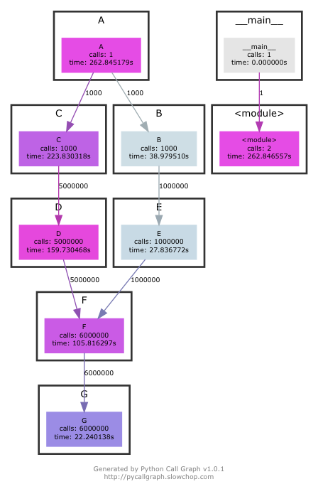
SnakeViz
Summary SnakeViz is a browser based graphical visualisation tool to display profiles using Icicle and Sunburst plots. It also includes IPython line and cell magics that can help to directly profile single line or code blocks and then visualise them. SnakeViz currently only works with files produced by cProfile (and not profile module). SnakeViz may not work with large, complex profile data but provide options to simplify plot by adjusting the cutoff and call-chain limits.
Compatibility Python2/Python3
Documentation User Guide, GitHub
Example First we generate profile using cProfile module and then simply launch snakeviz to visualize the data into browser:
|
1 2 3 4 5 |
$ python -m cProfile -o profile.pstats sample.py Execution time : 4.87 sec $ snakeviz profile.pstats |
The output is similar to other callgraph profilers with options to customise the visualisations directly in the browser: 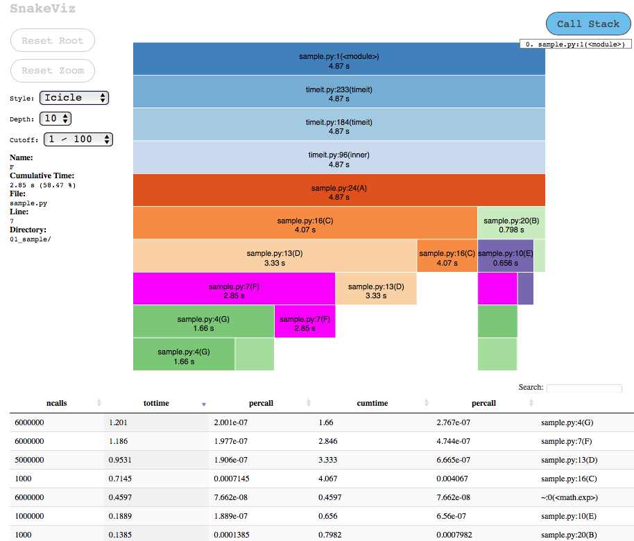
vprof
Summary vprof is a visual profiler that provides rich and interactive visualisations of different performance characteristics. One can generate plots like CPU flame graph, memory usage graph with process memory consumption after execution of each line and code heatmap. It can be also used in remote connection mode where vprof server launched in remote node can be connected with local visualisation client. You can see this example demonstrating remote mode with Flask web application.
Compatibility Python3.4+
Documentation README, GitHub
Note Safari shows flame graph upside down (because of SVG transform attributes), use Chrome and Firefox instead.
Example In below example I have launched profiler with all profiling options (memory, flamegraph and code heatmap). As you can see with the execution times, the memory profiling and heatmap profiling takes significant time. Also, profile.json of 3.2GB generated and took long time to write. Obviously the reading / rendering of this was stuck for long time. I gave up on memory profiling.
|
1 2 3 4 5 6 7 8 9 10 11 12 13 14 15 |
$ vprof -c cmh sample.py --output-file profile.json Running MemoryProfiler... Execution time : 357.11 sec Running FlameGraphProfiler... Execution time : 2.25 sec Running CodeHeatmapProfiler... Execution time : 67.42 sec $ du -h profile.json 3.2G profile.json $ vprof --input-file profile.json Starting HTTP server... |
The toy example we are using is very simple and hence the output doesn't look that impressive:
PyFlame
Summary PyFlame is a high performance profiling tool developed by Uber. It is implemented in C++ and uses statistical sampling techniques (over deterministic profiling) to keep profiling overhead low. Pyflame can take snapshots of applications without any source instrumentation. This is very helpful especially with large applications where modifying source code is not straightforward / time consuming. It fully supports profiling multi-threaded applications and also supports profiling services running under containers.
Compatibility Python2/Python3
Documentation User Guide, GitHub, Uber Blog
When To Use If you are profiling large, complex application, PyFlame is an effective tool for understanding the CPU and memory characteristics of long running applications in production environment. Note that PyFlame doesn't work on OSX or Windows platform.
Example PyFlame can be attached to already running process, or application can be profiled from start to finish as:
|
1 2 3 4 5 6 7 8 9 10 11 |
# attach to process PID 1024 for duration of 60 seconds and sample every 0.05 seconds $ pyflame -s 60 -r 0.05 -p 1024 .... $ pyflame --rate=0.005 -o profile.txt -t python sample.py Execution time : 1.97 sec # convert profile.txt to a flame graph flamegraph.pl < profile.txt > profile.svg |
This will generate flamegraph below:
plop
Summary plop is a low overhead, stack-sampling profiler for Python. Similar to PyFlame, it uses sampling technique and collect call stacks periodically. It allows to turn on/off profiling in a live process, see example usage of of start() and stop() APIs in this example. Plop has web based viewer implemented using Tornado and d3.js to display call graph. One can also generate profile output in flamegraph format (see below example).
Compatibility Python2/Python3
Documentation README, GitHub
Example To profile an entire Python application and then to generate flamegraph, one can do:
|
1 2 3 4 5 6 7 8 |
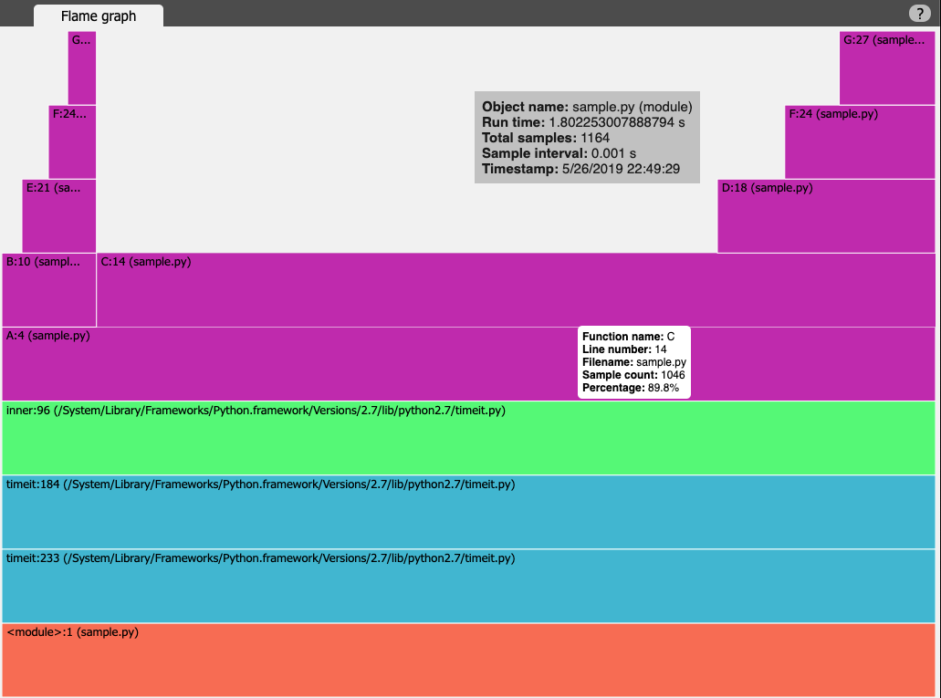
$ python -m plop.collector --interval 0.005 --format=flamegraph sample.py Execution time : 1.92 sec profile output saved to profiles/sample.py-20190526-1220-15.flame overhead was 2.59909926161e-05 per sample (0.00519819852323%) $ flamegraph.pl < profiles/sample.py-20190526-1220-15.flame > profile.svg |
This will generate flamegraph below:
Py-Spy
Summary Py-Spy is a sampling profiler written in Rust. It is inspired from rbspy and shows where program is spending time without need of restarting the application or modifying the application source code. Most of Python profilers modify application execution in some way: profiling code is typically run inside target python process which often slow down application execution. To avoid this performance impact, Py-Spy (and PyFlame) doesn't run in the same process as the profiled Python program. Because of this, Py-Spy can be used in production environment with little overhead.
Compatibility Python2/Python3
Documentation GitHub
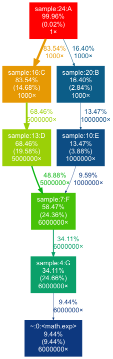
Example Similar to PyFlame, Py-Spy can attach to already running program or profile application from start to end. Py-Spy works by reading memory from a different python process and hence, in many case, you might need to execute profiler as a root user (with sudo or similar) depending on your OS and system settings. By default visualisation is a top-like live view:
|
1 2 3 4 5 6 7 8 9 10 11 12 13 14 15 16 17 18 19 20 21 22 23 24 25 26 27 |
$ sudo py-spy -- python sample.py Collecting samples from 'python sample.py' (python v2.7.12) Total Samples 100 GIL: 0.00%, Active: 100.00%, Threads: 1 %Own %Total OwnTime TotalTime Function (filename:line) 31.11% 31.11% 0.300s 0.300s G (sample.py:28) 24.44% 56.67% 0.250s 0.560s F (sample.py:25) 14.44% 55.56% 0.130s 0.500s D (sample.py:19) 10.00% 65.56% 0.090s 0.590s C (sample.py:16) 5.56% 5.56% 0.050s 0.050s C (sample.py:15) 5.56% 27.78% 0.080s 0.350s B (sample.py:12) 4.44% 21.11% 0.060s 0.260s E (sample.py:22) 1.11% 1.11% 0.010s 0.010s B (sample.py:11) 1.11% 1.11% 0.010s 0.010s E (sample.py:21) 1.11% 1.11% 0.010s 0.010s G (sample.py:27) 1.11% 1.11% 0.010s 0.010s F (sample.py:24) 0.00% 28.89% 0.000s 0.360s A (sample.py:6) 0.00% 100.00% 0.000s 1.00s inner (timeit.py:100) 0.00% 100.00% 0.000s 1.00s <module> (sample.py:30) 0.00% 100.00% 0.000s 1.00s timeit (timeit.py:237) 0.00% 100.00% 0.000s 1.00s timeit (timeit.py:202) 0.00% 71.11% 0.000s 0.640s A (sample.py:8) </module> |
But one can also generate flamegraph:
|
1 2 3 4 5 6 |
$ sudo py-spy --flame profile.svg --dump --function --rate 200 --duration 5 --nonblocking -- python sample.py Sampling process 200 times a second for 5 seconds Wrote flame graph 'profile.svg'. Samples: 370 Execution time : 1.85 sec |
which will generate flamegraph below:
And I will end this part-I with an unusual candidate:
pylikwid
Summary pylikwid is a python interface for LIKWID. LIKWID is a tool suite of command line applications that helps to measure various hardware counters with predefined metrics. It is used for low level performance analysis and works with Intel, AMD and ARMv8 processors.
Compatibility Python2/Python3
Documentation README, GitHub
When To Use It is not python profiler per say but if you are interested in low level performance analysis then it is a handy tool. For example, you are calling C/C++ library from Python application and want to analyse different hardware metrics.
Example Here is an example from the project website demonstrating use of LIKWID Marker API from Python:
|
1 2 3 4 5 6 7 8 9 10 11 12 13 14 15 16 17 18 19 20 |
#!/usr/bin/env python import pylikwid pylikwid.init() pylikwid.threadinit() liste = [] pylikwid.startregion("LIST_APPEND") for i in range(0,1000000): liste.append(i) pylikwid.stopregion("LIST_APPEND") nr_events, eventlist, time, count = pylikwid.getregion("LIST_APPEND") for i, e in enumerate(eventlist): print(i, e) pylikwid.close() |
Once python application is instrumented, we can run it under standard likwid-perfctr tool to measure the hardware counters. For example, in below case we are measuring L2 to L3 cache data transfer by pinning process to Core 0:
|
1 2 3 4 5 6 7 8 9 10 11 12 13 14 15 16 17 18 19 20 21 22 23 24 25 26 27 28 29 30 31 32 33 34 35 36 37 38 39 40 41 42 43 44 45 46 47 48 49 50 51 |
$ likwid-perfctr -C 0 -g L3 -m ./test.py -------------------------------------------------------------------------------- CPU name: Intel(R) Core(TM) i7-4770 CPU @ 3.40GHz CPU type: Intel Core Haswell processor CPU clock: 3.39 GHz -------------------------------------------------------------------------------- (0, 926208305.0) (1, 325539316.0) (2, 284626172.0) (3, 1219118.0) (4, 918368.0) Wrote LIKWID Marker API output to file /tmp/likwid_17275.txt -------------------------------------------------------------------------------- ================================================================================ Group 1 L3: Region LIST_APPEND ================================================================================ +-------------------+----------+ | Region Info | Core 0 | +-------------------+----------+ | RDTSC Runtime [s] | 0.091028 | | call count | 1 | +-------------------+----------+ +-----------------------+---------+--------------+ | Event | Counter | Core 0 | +-----------------------+---------+--------------+ | INSTR_RETIRED_ANY | FIXC0 | 9.262083e+08 | | CPU_CLK_UNHALTED_CORE | FIXC1 | 3.255393e+08 | | CPU_CLK_UNHALTED_REF | FIXC2 | 2.846262e+08 | | L2_LINES_IN_ALL | PMC0 | 1.219118e+06 | | L2_TRANS_L2_WB | PMC1 | 9.183680e+05 | +-----------------------+---------+--------------+ +-------------------------------+--------------+ | Metric | Core 0 | +-------------------------------+--------------+ | Runtime (RDTSC) [s] | 0.09102752 | | Runtime unhalted [s] | 9.596737e-02 | | Clock [MHz] | 3.879792e+03 | | CPI | 3.514753e-01 | | L3 load bandwidth [MBytes/s] | 8.571425e+02 | | L3 load data volume [GBytes] | 0.078023552 | | L3 evict bandwidth [MBytes/s] | 6.456899e+02 | | L3 evict data volume [GBytes] | 0.058775552 | | L3 bandwidth [MBytes/s] | 1.502832e+03 | | L3 data volume [GBytes] | 0.136799104 | +-------------------------------+--------------+ |
At the beginning CPU information is printed followed by hardware events and then different metrics for L3 cache. See the documentation of likwid-perfctr to interpret the results.
Thats all for this post. In Part-II I plan to cover: Intel VTune Amplifier, Arm MAP, pprofile, StackImpact Python Profiler, GreenletProfiler, Tracemalloc, vmprof, Python-Flamegraph, Pyheat, Yappi, profimp, PyVmMonitor , tuna and austin
-
Is Python faster and lighter than C++? stackoverflow ↩
-
Speed comparison with Project Euler: C vs Python vs Erlang vs Haskell stackoverflow ↩