Performance Engineering

Sunday, 7th April 2024: Back in September 2013, when I started my journey at the Blue Brain, I was navigating relatively large codebases for the first time. I was eager to gain a comprehensive understanding of code structures, their execution workflow, and performance aspects. During this period I started using Intel Vtune with xdot/gprof2dot and found it extremely useful. With this combination, I could generate detailed execution call graphs of applications and then sit together to deep dive into both the structural and performance aspects of the code with the senior engineers. More than 10 years have passed, and there are now many more tools available. However, I still find the workflow of Vtune + xdot useful from time to time. While others have written about gprof2dot/xdot, I thought it would still be helpful to convert my scattered notes into a blog post, especially touching on some of the specifics related to High-Performance Computing (HPC). And this short blog post precisely serves that purpose.

Background & Motivation

Working on large codebases with hundreds of thousands of lines of code is not an easy task. In many situations, such codebases have developed over a long period, and we might have access to only a few experts with a detailed understanding of the entire codebase. In scientific applications, the absence or scarcity of developer documentation is a common issue. In such situations, onboarding a new engineer is more than challenging. From the tools side, we commonly employ different strategies, for example: 1) employ modern IDEs and static analysis tools to explore the code in a better way 2) use runtime tools with a top-down approach to understanding the high-level structure of the application, or a bottom-up approach to understand specific functionality by focusing on a particular piece of code 3) use data flow analysis technique to identify key data structures and track how they are passed and updated in the key parts of the code.

Depending on the nature of the codebase (programming languages, parallel programming models), target platform, and runtime environment, implementing the aforementioned techniques may vary in difficulty. For instance, static code analysis may prove ineffective when dealing with applications composed of a mixture of languages like C++, Fortran, Python, and DSLs. Furthermore, runtime analysis tools may not be available on a target platform or support programming models like MPI, which is widely used in the area of High Performance Computing.

One specific scenario I have frequently seen while tackling new projects, whether for development or performance engineering purposes, is gaining a comprehensive understanding of the runtime behavior of the code. This entails delving into both the high-level structure of the application and conducting a deep dive into specific sections of the code. This multifaceted approach is essential because optimizing performance necessitates grasping the overall picture of the application before delving into the optimization of specific code parts.

Various profiling tools are readily available on the Linux platform, including specialized ones for HPC applications (see Summary of Profiling Tools for Parallel Applications). During 2013, I was specifically looking for call graphs to gain a better high-level understanding, but for one reason or another, I found the reports generated from some of the commonly used tools unsatisfactory. For instance, gprof was painfully slow with complex codes, perf wasn't available on HPC clusters (and still often the case), and the call path profiles from TAU didn't look that great. Later that year I stumbled upon gprof2dot which gained support for importing Vtune's gprof-like output. The reason I found the combination of Intel's Vtune and gprof2dot quite effective is that Vtune had everything one would need, especially a decade ago when most of the HPC systems were powered by x86_64 CPUs, to profile HPC applications: support for prominent parallel programming models, low overhead on application runtimes, APIs to start/pause/resume profiling for interesting code sections, the ability to adjust sampling frequencies, etc. I could export the Vtune's profile results into a gprof-like format and then use gprof2dot or xdot to generate call graphs. I was quite happy with the insight I was able to generate in a short amount of time!

That's enough dwelling on past memories. Let's see how to use these tools in practice!

Installation

Installing gprof2dot and xdot is a straightforward process as they are available as Python packages via pip. However, it's worth noting that gprof2dot requires the Graphviz dependency, while xdot has additional dependencies like PyGObject:

After installing the dependencies, you can proceed to install gprof2dot and xdot using pip:

Once installed, you can verify that the gprof2dot and xdot commands are available in your shell:

When it comes to installing profiling tools like Intel Vtune or Perf, better if refer to the latest instructions related to your platform. Here are the commands that I used to install them on my Ubuntu desktop:

You can check if the Vtune and perf are working:

If both commands finish without errors, then we have everything set up!

Sample Application

Before diving into real-world production applications, let's start with a straightforward example with the code snippet given below:

Clear and concise, isn't it? The code structure mirrors a typical structure of some scientific applications, featuring an initialization routine for loading input data, a simulation routine responsible for executing a specified number of timesteps, and a finalization routine for cleanup and result output. While the MPI aspect can be ignored, it's included to offer insight into an MPI-based execution workflow. To ensure meaningful profiling timings, we have introduced a dummy_work()" routine, dedicated to consuming some compute cycles.

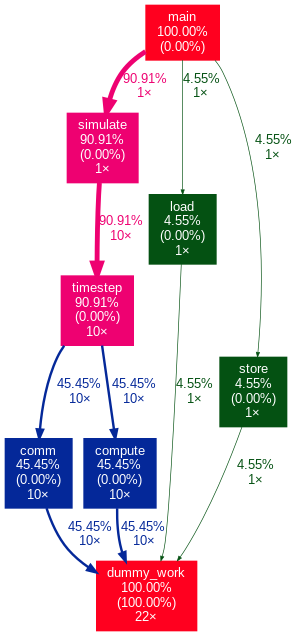
If we visualize the execution workflow as a call graph, our drawing should look like the below:

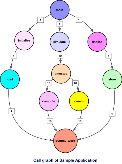
The numbers accompanying the edges denote the frequency of function calls. Our objective with profiling tools is to automatically generate such a structured representation to provide insight into an application and its execution workflow.

Intel Vtune and gprof2dot In Action

Assuming Intel VTune is already set up, we can compile and generate a profile for our sample application using the following steps. Let's begin by focusing on serial, non-MPI execution:

Using --report=gprof-cc CLI option, we obtain sample_profile.txt in the gprof-like format:

We can then use gprof2dot to generate a call graph as follows:

For an explanation of the CLI arguments, refer to the "Miscellaneous" section. The gprof2dot generates a DOT file, and we utilize the dot utility to convert it to an image. Upon inspecting sample_profile.png, you'll observe:

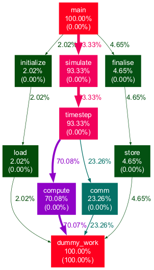
Pretty neat, isn't it? It aligns with our previous drawing! Each node displays inclusive and exclusive time (in parentheses) as a percentage of the total application runtime. The thickness of edges also corresponds to the amount of execution time spent in a specific call chain. By experimenting with the CLI arguments, you can produce highly informative plots tailored to the intricacies of complex applications!

MPI Applications

If you are familiar with utilizing Intel VTune for HPC applications, you are likely familiar with the amplxe-cl or vtune CLI. Let's run our example with four ranks and collect hotspot profile using commands below:

Depending on your node configuration and execution environment, VTune will generate multiple results directories, one per compute node. For instance, if you allocated 4 nodes with 1 rank per node, VTune will create 4 different directories, each corresponding to a compute node:

Depending on the nature of the application, you may need to analyze profile results from either a single compute node or a group of compute nodes. For illustrative purposes, let's create call graphs for the initial and final ranks executed on the compute nodes identified by the hostnames r1i5n18 and r1i5n21, respectively:

Note the inclusion of the --leaf=dummy_work CLI argument, which restricts the displayed nodes to those reaching the dummy_work() function. This indirectly filters out functions from external libraries such as MPI. Below, you can see the resulting call graphs for the two ranks displayed side by side:

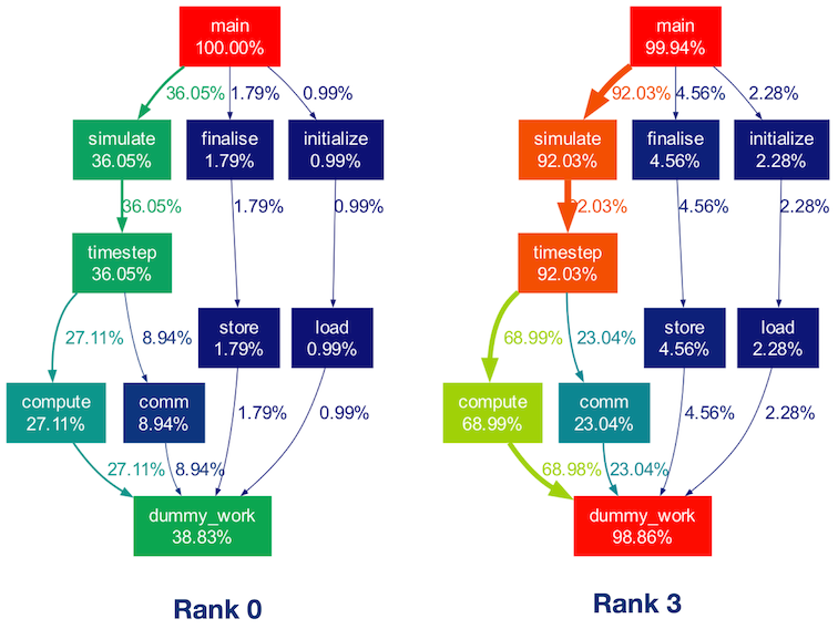
While the execution workflow remains consistent across ranks, differences in execution times are noticeable in the above two call graphs. This discrepancy arises because the dummy_work() function consumes more time for higher ranks. Additionally, Rank 0 spends a significant portion of its time in MPI initialization and finalization, causing the time spent in children of the main() function to not sum up to 100%.

Production Application

The example provided in the previous section demonstrated the usage of Vtune + gprof2dot in analyzing serial as well as MPI applications. Now, let's apply this approach to a real-world production application: NEURON.

Over the course of three decades, NEURON has evolved into an important tool for computational neuroscience, facilitating the simulation of electrical activity in morphologically detailed neuron network models. Having been deeply involved in its advancement over the past decade, I can attest to the complexity inherent in the NEURON codebase. It's a complex mix of C, C++, and Python code, intertwined with its own domain-specific language (NMODL) and a HOC interpreter. Navigating NEURON's extensive codebase, particularly with the inclusion of the NMODL DSL language and HOC interpreter, can be a daunting task. Using the Vtune + gprof2dot, we will see if we can get valuable insights into understanding code structure as well as its execution workflow.

We will use the same workflow that we employed for the MPI application in the previous section. I am going to use the benchmark that we have put together to showcase the computational characteristics of the Cortex and Hippocampus brain regions. We won't delve into benchmark-specific details and CLI parameters. The way in which we run this benchmark with the NEURON simulator is as follows:

Next, let's profile the execution under Vtune and generate a report:

Now, let's convert that report to a call graph using gprof2dot:

In the previous example, we used -Tpng to generate the call graph as PNG images. However, in production applications, the graph might be too large to fit within Cairo's maximum bitmap size of 32767x32767 pixels. As a result, dot will scale the image (as shown in the above console output) and the resulting images may not be readable. To address this issue, we can instruct dot to generate SVG output instead:

If we examine the generated call graph simply via web browser (or DOT file via the xdot, see the next section), we should see below callgraph:

Indeed, the graph appears quite complex! While it's still possible to navigate through this detailed graph, it's unlikely that you want to see every node for which profile data is collected (implied by the --node-thres=0 --edge-thres=0 CLI arguments). Let's remove those CLI arguments to filter out nodes with lower execution time. Additionally, we'll use the --root=psolve CLI argument to focus the call graph on the main solver entry point routine psolve() in NEURON:

This yields a more manageable call graph:

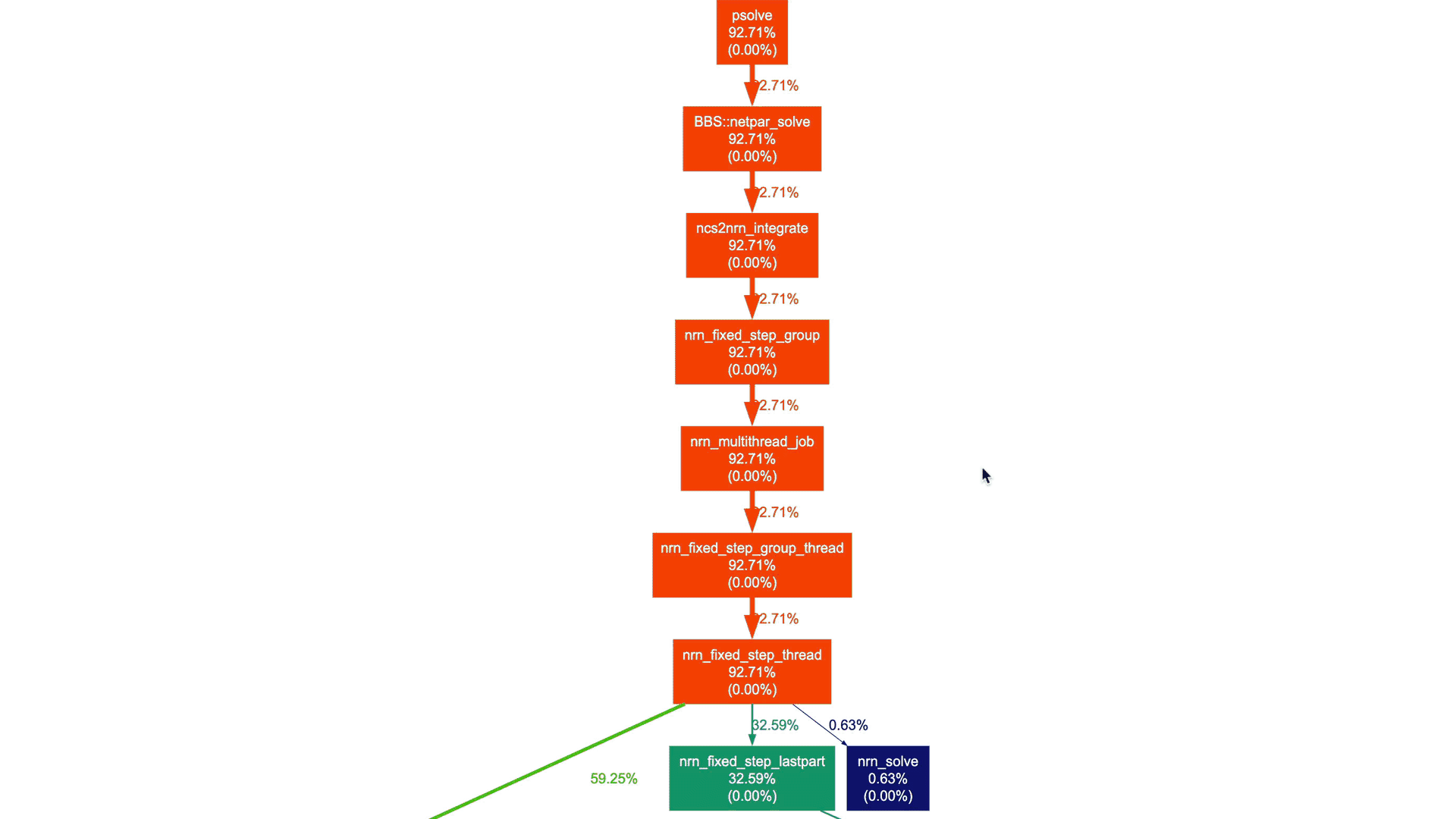
We don't need to delve into NEURON-related details and understand the actual call graph. However, as a NEURON developer, I can certainly say that these high-level call graphs can be extremely useful for gradually gaining an understanding of the application structure and beginning to explore performance aspects.

Miscellaneous Topics And Insights

xdot: Interactive Viewer for DOT Files

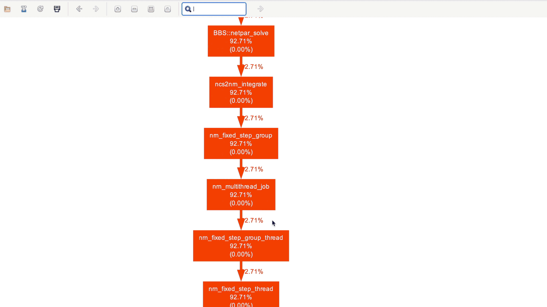
In the case of production applications with large and intricate call graphs, refining the call graph to focus on specific code sections can be cumbersome. This is where xdot comes to the rescue! It offers an intuitive graphical interface for dynamically exploring and interacting with call graphs in DOT format. With xdot, one can easily navigate, zoom in, search, and inspect individual nodes and edges. This helps in analyzing and understanding complex graph structures. Here is the xdot in action for the NEURON callgraph that we generated earlier:

Useful CLI arguments of `gprof2dot

Here is a summary of CLI arguments that I find useful while using gprof2dot:

• --format=axe: format of the input file (e.g. axe for Vtune)
• --node-thres=0: eliminate nodes below this threshold [default: 0.5].
• --edge-thres=0: eliminate edges below this threshold [default: 0.1]
• --strip: strip function parameters, template parameters, and const modifiers from function names.
• --depth=X: show only descendants or ancestors until the specified depth.
• --root=name: show only descendants of specified root function.
• --leaf=LEAF: prune call graph to show only ancestors of specified leaf function

Adjusting Sampling Frequency for Granular Profiles

In certain scenarios, increasing the sampling frequency when generating profiles can be advantageous, especially for capturing functions that execute very quickly. This approach allows us to create a comprehensive profile where most of the execution workflow information is captured. Subsequently, we can selectively generate call graphs for specific code sections of interest. In Intel VTune 2024, we can adjust the sampling frequency using CLI options like the following:

Note that the sampling interval is fixed for the software sampling mode, which means we must use the hardware sampling mode to adjust the sampling frequency. However, it's important to mention that using hardware event-based sampling requires special permissions for the Vtune driver. You can refer to the relevant documentation for more information.

Is Intel VTune Necessary? Why Not Linux Perf or Simply Gprof?

As mentioned earlier, Intel VTune is not the only option. gprof2dot supports various other profiling tools including gprof, perf, oprofile, callgrind, etc. However, Intel VTune offers support for commonly used programming models like MPI and OpenMP in the HPC domain. Additionally, it's often more readily available on HPC clusters compared to Linux perf. While gprof may suffice for demo applications, it quickly becomes impractical for complex, production applications due to its high overhead resulting from compiler instrumentation techniques.

If you have access to Linux perf, you can easily perform profiling and generate a call graph with the following command:

In the README file here, you can find various examples.

Using gprof with MPI Applications

For simple codebases like our demo application demonstrated previously, gprof could work:

Executing this should produce four distinct gprof profile data files:

Now, we can generate call graph using gprof2dot as:

This generates a plot resembling:

Since gprof relies on compiler instrumentation rather than sampling like Vtune and perf, it provides precise call counts in the generated profiles.

Profiling only Regions of Interest

In the context of production applications, there may be instances where we wish to exclude certain code regions from profiling, such as initialization procedures. For example, in the case of NEURON, initialization involves functions for loading model data and HOC interpreter execution, which is not often important for performance analysis. To address this, Intel Vtune offers two options:

• Use the -resume-after=<double> CLI option to commence profiling after a specified duration.
• Use the -start-paused option and then incorporate itt_resume() and itt_pause() APIs within the application to control data collection at runtime.

References

Using tools like gprof2dot and xdot is straightforward, especially if you are already familiar with profiling tools such as perf, Vtune, gprof, etc. Generating profiles and importing them into these tools is relatively simple. The documentation in gprof2dot and xdot repositories should provide you with more than enough information:

• gprof2dot GitHub repository: https://github.com/jrfonseca/gprof2dot
• xdot GitHub repository: https://github.com/jrfonseca/xdot.py

Credits

gprof2dot and xdot exemplify how even small tools can be significantly useful. Looking into their GitHub history, I see that José Fonseca initiated the development of these tools nearly 17 years ago. All credit to José Fonseca for creating these invaluable tools. Thank you, José!