Performance Engineering

March 2020: I was planning to write about CPU microarchitecture analysis for a long time. I started writing this post more than a year ago, just before the beginning of COVID-19. But with so many things happening around (and new parenting responsibilities 👧), this got delayed for quite a long time. Finally getting some weekend time to get this out!

Like previous blog posts, this also became longer and longer as I started writing details. But I believe this gives a comprehensive overview of LIKWID capabilities with the examples and can be used as a step-by-step guide. The section about hardware performance counters is still very shallow and I hope to write a second part in the future. I have added Table of Contents so that you can jump to the desired section based on your experience/expectation.

Table of Contents

• I. Introduction
  Start here to understand motivation and background about the LIKWID.
• II. Brief Overview of CPU Architecture
  Start here to get an idea of modern CPU architecture and common terminologies.
• III. What do we want to understand using LIKWID?
  Start here to know what we are going to achieve in this blog post.
• IV. Installing LIKWID
  Start here to begin with LIKWID installation and common issues.
• V. LIKWID In Practice
  Start here to understand how LIKWID can be used for various use cases.
  • 1. Understanding topology of a compute node : #threads, #cores, #sockets, #caches, #memories
  • 2. Understanding topology of a multi-socket node with GPUs
  • 3. Thread affinity domains in LIKWID
  • 4. How to pin threads to hyperthreads, cores, sockets or NUMA domains?
  • 5. likwid-bench : Microbenchmarking framework
  • 6. Understanding workgroups in the likwid-bench
  • 7. Understand structure and output of likwid-bench
  • 8. What is peak FLOPS performance of a CPU?
  • 9. Do we get better FLOPS with Hyper-Threading?
  • 10. What is memory bandwidth of a CPU? What role vectorisation play in bandwidth?
  • 11. How many cores are required to saturate bandwidth?
  • 12. Measuring impact from caches
  • 13. What is NUMA effect? How to quantify the impact?
  • 14. Changing CPU frequency and turbo mode
  • 15. How to measure power consumption?
  • 16. Measuring performance counters with ease!
  • 17. But, after all this, how can I analyse my own application?
• VI. Additional Resources
  See additional references that can be helpful to explore this further.
• VII. Credit
  Praise the fantastic developer team!

I. Introduction

Modern processors are complex with more cores, different levels of parallelism, deeper memory hierarchies, larger instruction sets, and a number of specialized units. As a consequence, it is increasingly becoming difficult to predict, measure, and optimize application performance on today's processors. With the deployment of larger (and expensive) computing systems, optimizing applications to exploit maximum CPU performance is an important task. Even though application developers are taking care of various aspects like locality, parallelization, synchronization, vectorization, etc., making optimal use of processors remains one of the key challenges. For low-level performance analysis, there are few vendor-specific tools available but if you are looking for a lightweight, easy-to-use tool for different CPU platforms then LIKWID must be on yout list!

LIKWID (Like I Knew What I am Doing) is a toolsuite developed at Erlangen Regional Computing Center (RRZE) over last ten years. It provides command-line utilities that help to understand thread and cache topology of a compute node, enforce thread-core affinity, manipulate CPU/Uncore frequencies, measure energy consumption and compute different metrics based on hardware performance counters. LIKWID also includes various microbenchmarks that help to determine the upper bounds of a processor performance. It supports Intel, AMD, ARM, and IBM POWER CPUs. The last release (v5) of LIKWID has added very basic support for NVIDIA GPUs. If you want to understand more about LIKWID and its architecture, this 2010 paper gives a good overview. Also, see resource section for other useful references.

I became familiar with LIKWID in 2014 when one of a master student from the LIKWID group started an internship in our group for performance modeling work. For large-scale performance analysis I often use a bunch of other profiling tools (see my list here) but LIKWID always comes in handy when need to look into microarchitecture details and tune single node performance.

Do You Want To Understand Your CPU Better? Then let's get started!

II. Brief Overview of CPU Architecture

With diverse architecture platforms, it is difficult to summarise modern CPU architectures in a blog post. And, it's not the goal of this post anyway! There are already excellent resources available. But, for the discussion here we would like to have a high-level understanding and common terminology in place. So, before jumping into the LIKWID, we will look at the high-level organization of compute node and processor architecture. Note that from one computing system to another and one CPU family to another, the organization and architecture details will be different. But the goal here is to highlight certain aspects that give an idea of what one should be aware of.

Compute Node Architecture

A compute node can be considered a basic building block of computing systems today. A node consists of one or more sockets. A socket is hardware on the motherboard where processor (CPU) is mounted. A processor has components like ALU, FPU, Registers, Control Unit, and Caches are collectively called a core of a processor. These components can be replicated on a single chip to form a multi-core processor. Each core can execute one or more threads simultaneously using hyper-threading technology. Each core has one or more levels of private caches local to the core. There is often a last-level cache that is shared by all cores on a processor. Each socket has main memory which is accessible to all processors in a node through some form of inter-socket link (see HT, QPI or UPI). If the processor can access its own socket memory faster than the remote socket then the design is referred to as Non-Uniform Memory Access (NUMA). A generalized sketch of a typical compute node is shown in the below figure. The number of sockets, cores, threads, and cache levels are chosen for simplicity.

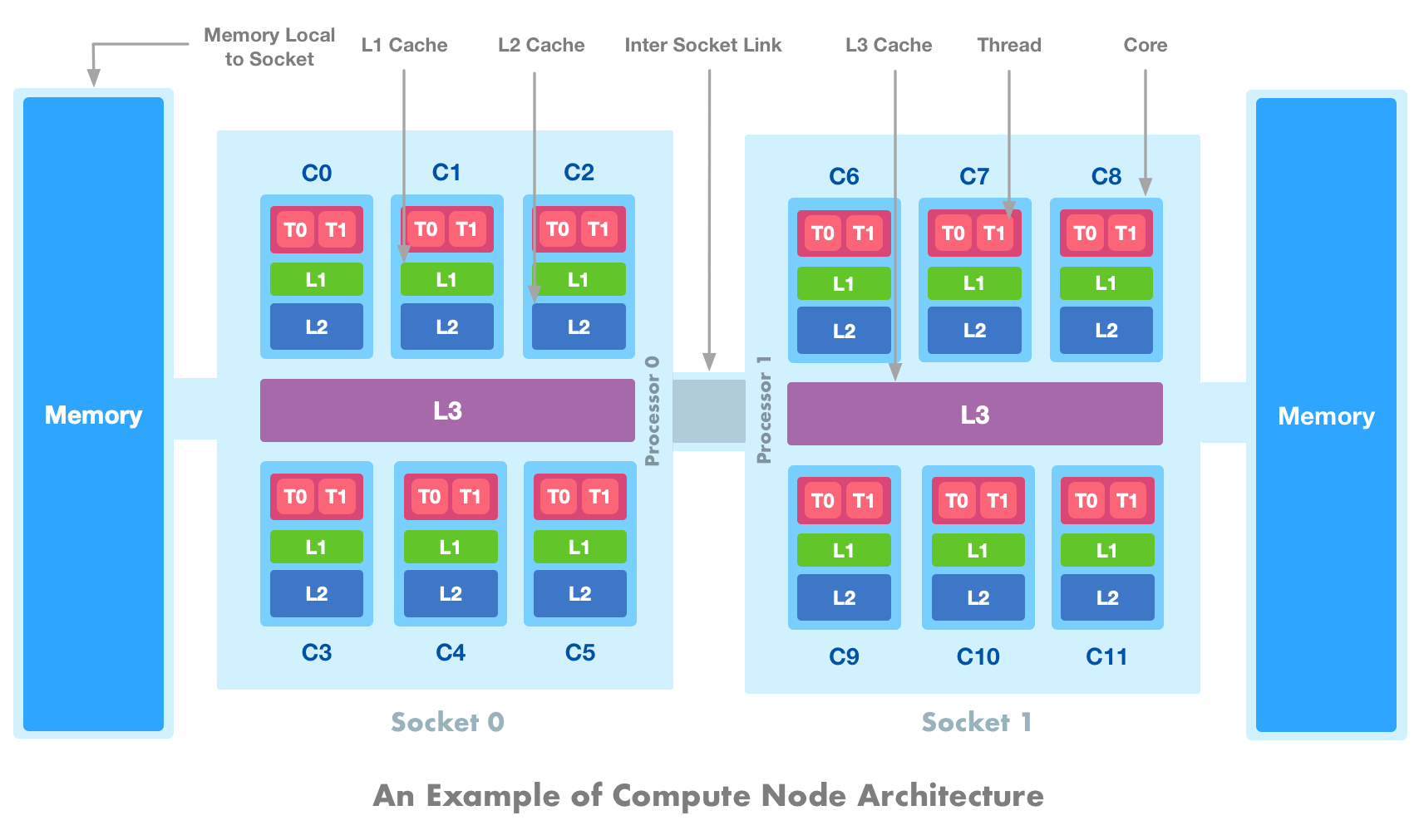
In the above figure, we have depicted a dual-socket system (Socket 0 and Socket 1) where each socket contains a 6-core processor (C0-C5 and C6-C11). Each core is 2-way SMT i.e. can execute two threads simultaneously (T0-T1). There are two levels of caches (L1 and L2) local to each core. There is also an L3 cache that is shared across all 6 cores on a single processor. Two sockets are connected by an inter-socket bus through which the entire memory is accessible. There are two NUMA domains and access to local memory on each socket is faster than accessing memory on a remote socket via inter socket link. Note that the cores and memories on a socket can be further subdivided into multiple sub-domains for improved core-to-memory access (e.g. using SubNUMA Clustering (SNC) on modern Intel CPUs).

CPU Core Architecture

Once we understand compute node architecture, the next step is to understand the microarchitecture of the individual processor and this is where the complexity comes in. A node architecture presented in the previous figure is quite generic across the systems. But, processor microarchitectures are quite diverse from one vendor to another or even from one processor generation to another. In this blog post, we are not going to look into performance bottlenecks within the CPU core and I plan to write a second part to cover this topic. But to get an idea of the individual processor and its functioning, let's take a look at the Intel Skylake processor core. Based on the Intel Press Workshop 2017 presentation, a simplified schematic representation of the core is shown below:

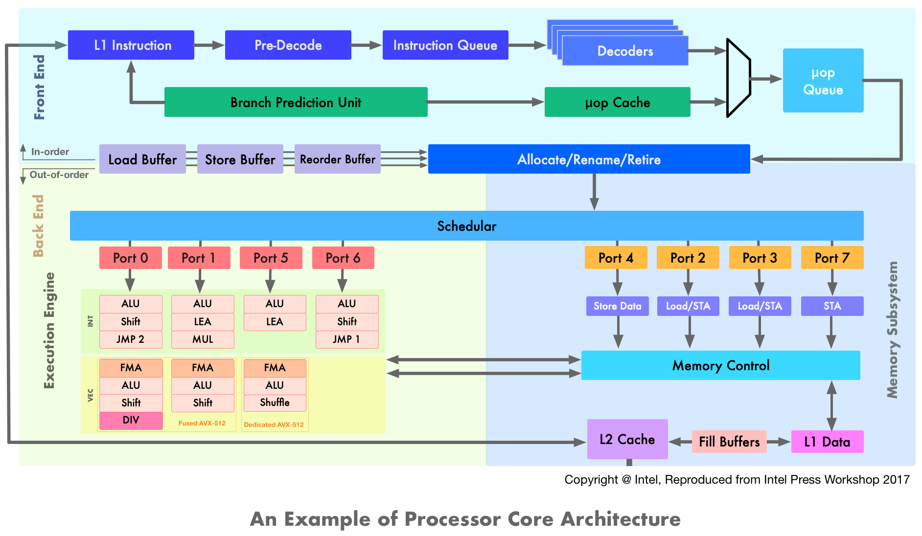
As highlighted in the three different color blocks, the processor core can be divided into three main parts: Front-End, Execution Engine (Back-End), and Memory Subsystem. Here is a brief overview of these building blocks:

• Front-End: An in-order issue front-end is responsible for fetching instructions from memory to instruction cache, decoding them, and delivering them to the Execution Engine. The instructions can be complex, variable in length, and may contain multiple operations. At the Pre-Decode buffer, the instructions boundaries get detected and then stored into Instruction Queue. Decoders pick the instructions and convert them into regular, fixed-length µOPs. As decoding complex instructions is an expensive task, the results are stored in µOP cache. The Allocate/Rename block reorders the µOPs to dataflow order so that they can be executed as their sources are ready and execution resources are available. The Retire unit ensures that the executed µOPs are visible according to the original program order. The scheduler store the µOPs which are waiting for execution and can dispatch a maximum of 8 µOPs per cycle (i.e. one per port).

• Execution Engine: An out-of-order, superscalar Execution Engine is responsible for the execution of µOPs sent by the scheduler. It consists of multiple Execution Units each dedicated to certain types of µOPs. Some Execution Units are duplicated to allow simultaneous execution of certain µOPs in parallel. The Execution Engine has support for Intel's AVX-512 instruction set which can perform 8 double or 16 single-precision operations per instruction. Note that AVX-512 fuses Port 0 and Port 1 (which are 256-bit wide) to form a 512-bit FMA unit. In the high-end Xeons, there is a second dedicated 512-bit wide AVX-512 FMA unit on Port 5. The Execution Engine also has connections to and from the caches.

• Memory Subsystem: The Memory Subsystem is responsible for memory load and store requests and their ordering. The µOPs related to data transfer are dispatched to Memory Subsystem by the Schedular via dedicated ports. Each core has a separate L1 cache for data and instruction whereas the L2 cache is shared for data as well as for instructions. Fill Buffer (FB) keeps track of outstanding cache misses and stores the data before loading into the L1 cache. The memory control unit manages the flow of data going to and from the execution units. On Skylake the memory subsystem can sustain two memory reads (Port 2 and Port 3) and one memory write (Port 4) per cycle. Port 7 handles the memory address calculation required for fetching data from the memory.

There are many other details involved in each part and it's out of the scope of this blog post to cover them in detail. If you want to dive into details, you can take a look at Intel 64 and IA-32 Architectures Optimization Reference Manual and wikichip.org.

III. What do we want to understand using LIKWID?

As application developers or performance engineers, we have heard a number of guidelines and recommendations in one or another form. For example, caches are faster, hyperthreading doesn't always help, memory bandwidth can be saturated by smaller core count, access to memory on remote NUMA node is slower etc etc. But, if doing X is slower than Y then the question is how much slower? The obvious answer "it depends" doesn't help that much. LIKWID doesn't provide direct answers to all these questions but provides a good framework to quantify the impact in a systematic way. In this blog post, using LIKWID, we are going to:

• Understand compute node topology including cores, caches, memories and GPUs
• Understanding how to pin threads to virtual cores, physical cores or sockets
• Measure performance of a core and a compute node
• Measure bandwidth using a core and a compute node
• Understand the effect of memory locality on performance
• Understand the effect of clock speed on performance
• Understand the effect of hyper-threading
• Measure energy consumption
• Measure hardware performance counters for flops, memory accesses
• Understand how CPU frequency can be changed along with turbo mode
• Understand how to analyze our own application

IV. Installing LIKWID

Secutiry Considerations In order to enable hardware performance counter analysis, access to model-specific registers (MSR) is required on the x86 platform. These MSR registers can be accessed via special instructions which can be only executed in protected mode or via device files on newer kernels (>= v2.6). By default, the root user has permissions to access these registers. One can install LIKWID with the root user but one has to consider security aspects especially on shared computing systems. An alternative approach is a solution based on access daemon, see this section in the official documentation. If you don't have root permissions on the system then you can use perf_event backend but that could be with limited features. See this documentation. For the sake of simplicity and easy setup we are installing with a root user here.

Installing LIKWID is easy on any Linux distribution. Apart from basic dependencies (like make, perl, zlib) other dependencies are shipped with the released tarballs. We can download and build LIKWID as:

Manual Installation

And now if we try to install as a normal user then we should get the following error:

This is because LIKWID is trying to change ownership of likwid-accessD daemon to get elevated permissions. As a normal user this it's not possible to change ownership to root. An easy way to avoid this error is to perform the install step using the root or sudo command:

Again, prefer this approach only after going through the security considerations (discussed here).

Lets now add the installation directory to PATH:

Spack Based Installation

If you are using Spack for building scientific software then you can install LIKWID as:

Note that as of today, Spack installs LIKWID with perf_event backend. So you have to make sure to update to the appropriate level in /proc/sys/kernel/perf_event_paranoid (see this documentation on kernel.org). If you have set up a separate Linux group for a set of users to use LIKWID with extra permissions then you have to set LIWKID_GROUP environmental variable and use setgid variant as:

Current Spack recipes set BUILDFREQ=false and BUILDDAEMON=false which means likwid-setFrequencies and access daemon likwid-accessD are not built. See the discussion in google group and GitHub issue.

Either with manual installation or Spack-based installation, we hope everything is installed correctly. Let's do a basic check:

Looks great! Both commands are finishing without any error. If you see any errors with the above commands then refer to the summary I posted in this GitHub issue. Here are some additional notes:

• To see various build options, take a look at config.mk. Commonly used options in config.mk are: COMPILER, PREFIX, ACCESSMODE, NVIDIA_INTERFACE, BUILDDAEMON, BUILDFREQ.
• LIKWID can be built on top of perf_event backend instead of native access. See details here.
• Instrumentation under likwid-bench can be enabled with an option INSTRUMENT_BENCH = true.
• If you are using LIKWID in a cluster and LIKWID is preinstalled then some advanced features might have been disabled (e.g. changing clock frequencies).

V. LIKWID In Practice

Instead of writing about each tool (which is already available via GitHub Wiki), we will try to address specific questions discussed in the Section 3 using different tools provided by LIKWID. Throughout this post, we are going to use a compute node with two Cascade Lake 6248 CPUs @ 2.5 GHz (20 physical cores each and hyperthreading enabled). For the next one section about node topology we will also use linux desktop with a Haswell 4790 CPU @ 3.0 GHz (4 physical cores and hyperthreading enabled).

1. Understanding topology of a compute node : #threads, #cores, #sockets, #caches, #memories

Before diving into performance analysis, first thing is to get a good understanding of the compute node itself. You might have used tools like numactl, hwloc-ls, lscpu or simply cat /proc/cpuinfo to understand the CPU and cache organization. But based on the platform and BIOS settings, information like CPU numbers could be different on the same compute hardware. LIKWID tries to avoid such discrepancies by using information from different sources like hwloc library, procfs/sysfs, cpuid instruction etc. and provides a uniform view via tool called likwid-topology. It shows the topology of threads, caches, memories, GPUs in a textual format.

Let's start with a Linux desktop with a Haswell CPU. Using lscpu command we can find out various properties as:

This is a single socket, quad-core CPU with hyperthreading enabled (i.e. 8 virtual cores). As there is a single socket and no SNC is enabled, there is only one NUMA domain. If we want to find out how threads and caches are organized then we can do:

Here we can see CPU 0 and CPU 4 are mapped to same physical core Core 0. They share all data instruction caches (0:0:0:0 represent L1d:L1i:L2:L3 which is 0th L1 data cache, L1 instruction cache, L2 data cache and L3 data cache). Maximum and minimum CPU freqency along with CPU status (online or offline) is shown as well.

Using likwid-topology we can get the similar information in a more intuitive way. For example, here is the output of likwid-topology command on the same node:

If we compare the above information with lscpu output then most of the information is self-explanatory. Note that we have added annotations of the form (X) on the right to describe various sections. Here is a brief summary:

• (1) shows CPU information and base frequency. (stepping level indicates a number of improvements made to the product for functional (bug) fixes or manufacturing improvements).
• (2) shows information about the number of sockets, number of physical cores per socket, and number of hardware threads per core.
• (3) shows information about the association of hardware threads to physical core and sockets. It also shows if a particular core is online or offline. (You can mark particular core online or offline by writing 0 or 1 to /sys/devices/system/cpu/cpu*/online).
• (4) shows information about sockets and which hardware threads or cores it contains.
• (5) shows different cache levels, their sizes, and how they shared by hardware threads or physical cores. For example, Level 1 cache level is 32 kB and each physical core has a separate 32 kB block. This is indicated by cache groups like ( 0 4 ) which are two hardware threads of physical Core 0.
• (6) shows NUMA domain information and memory size. As this node has a single NUMA domain, Domain 0 comprises all cores and NUMA distance is minimum i.e. 10.
• Finally, (7) shows graphical topology information which is easy to comprehend. The first physical core has two hyperthreads (0, 4) and it has a private L1 cache of 32 KB and a private L2 cache of 256 KB. The last level cache of 8 MB is shared across all 4 cores. This is especially helpful when you have a multi-socket compute node and you don't need to scan all textual output.

You can find additional information about the likwid-topology tool here.

2. Understanding the topology of a multi-socket node with GPUs

likwid-topology becomes more handy and intuitive as compute node gets more complex. Let's look at an example of a dual-socket compute node with 4 NVIDIA GPUs. The output is trimmed for brevity:

The above output is familiar to us. We will highlight major differences due to dual socket and GPUs:

• (1) shows that there are two sockets with 20 physical cores each. Each physical core has two hardware threads as hyperthreading is enabled.
• (2) shows hardware thread topology. Physical cores 0 to 19 are part of the first socket and 20 to 39 are part of the second socket. The hardware threads from 40 to 59 and 60 to 79 represent hyperthreads corresponding to the first and second socket respectively.
• (3) shows that there are two NUMA domains corresponding to two sockets. The Distances metric shows that there is extra cost access memory across NUMA domains. This also confirms that there are two different physical NUMA domains.
• (4) shows information about GPUs available on the node. There are four V100 NVIDIA GPUs and various hardware properties like L2 cache size, memory size, frequency are shown.
• (5) shows the graphical topology of the node. This is a quick way to capture the overall topology of the node. You might have noticed that the GPUs are not shown in this graphical topology.

This should have provided you a good overview of what to expect from likwid-topology. You can look at more examples on LIKWID Wiki page. Note that in order to detect GPUs, GPU support needs to be enabled at install time and CUDA + CUPTI libraries must be available (e.g. using LD_LIBRARY_PATH).

3. Thread affinity domains in LIKWID

Every few months I return to LIKWID and forget or mix naming conventions. So in the next few sections, we will look into some of the common terminology and syntax used with LIKWID.

LIKWID has the concept of thread affinity domains which is nothing but a group of cores sharing some physical entity. Here are four different affinity domains:

• N : represents a node and includes all cores in a given compute node
• S : represents socket and include all cores in a given socket
• C : represents last level cache and include all cores sharing last level cache
• M : represents NUMA domain and includes all cores in a given NUMA domain

These domains can be well explained by an example. One can use likwid-pin tool to list available domains on a given compute node:

In the above example, each physical core is shown with two hyperthreads as hyperthreading is enabled. For example, (0,40) represents the physical core 0, (1,41) represents the physical core 1, and so on. The N represents the entire compute node comprising all physical and logical cores from 0 to 69. The S0 and S1 represent two sockets within the compute node N. The L3 cache is shared by all cores of individual sockets and hence there are two groups C0 and C1. Each socket has local DRAM and hence there are two memory domains M0 and M1.

4. How to pin threads to hyperthreads, cores, sockets or NUMA domains

Pinning threads to the right cores is important for application performance. LIKWID provides a tool called likwid-pin that can be used to pin application threads more conveniently. It works with all threading models that use Pthread underneath and executables that are dynamically linked.

likwid-pin can be used as:

where pin-options are CPU cores specification. Lets look at the examples of <pin-options> that will help to understand the syntax better:

• N:0-9 : represent 10 physical cores in a node (notice N which decide domain to entire node). As we have two sockets in a node, the first 5 physical cores from each socket will be selected. Note that for all logical numbering schemes physical cores are selected first.
• S0:0-9 : represent the first 10 physical cores in the first socket (notice S0 which decide 0th socket in the node).
• C1:0-9 : represent the first 10 physical cores sharing shared L3 cache. This will be the same as S1:0-9 i.e. 10 physical cores in the second socket.
• S0:0-9@S1:10-19 : represent first 10 physical cores from the first socket S0 and the last 10 physical cores from the second socket S1. The @ can be used to chain multiple expressions.
• E:S0:10 : represents expression based syntax where 10 cores from the first socket with compact ordering. This means, as hyperthreading is enabled, the first 5 physical cores are selected and threads are pinned to each hyperthread. The expression based syntax has form E:<thread domain>:<number of threads>.
• E:S0:20:1:2 : represents expression based syntax of form E:<thread domain>:<number of threads>:<chunk size>:<stride>. In this case, in the first socket S0, we are selecting 1 core (as chunk size) after every 2 cores (as stride) and in total 20 cores. If we look at the output of likwid-pin shown above, this means we are selecting 0,1,2,3,4....19 which is all physical cores in the first socket i.e. S0:0-19.
• M:scatter : scatter threads across all NUMA domains. First physical cores from each NUMA domain will be selected alternatively and then hyperthreads on both sockets. In above example, it will result into following selection: 0,20,1,21,2,22....19,39,40,60,41,61...59,79.
• 0,2-3 : represent CPU cores with Ids 0, 2 and 3. Note that we are not using domain prefix here but directly specifying physical CPU Ids and hence this is called physical numbering scheme.

The reason for covering these all syntaxes in one section is that they used in this blog post but also in other LIKWID tutorials. So this section pretty much covers all necessary pinning-related syntaxes that one needs to know.

5. likwid-bench : A microbenchmarking framework

One of the tools that make LIKWID quite unique compared to other profiling tools is likwid-bench. Like older LLCbench and LMbench tools, the goal of likwid-bench is to provide microbenchmarking tool that can help to gain insight into the microarchitecture details. It also serves as a framework to easily prototype multi-threaded benchmarking kernels written in assembly language. We will not go into too many details in this blog post but you can read the details in this manuscript and the wiki page.

We can list available microbenchmarks using -a option:

Note that the above list is not complete but we are only showing main benchmark categories. Each benchmark is implemented with different instruction sets (e.g. SSE, AVX2, AVX512, ARM NEON, Power VSX, ARM SVE) depending upon the target ISA. You can see the platforms and their implementation under bench sub-directory. You can get information about each kernel using likwid-bench -l command. In the next sections, we will use these microbenchmarks to measure performance metrics like flops and memory bandwidth.

6. Understanding workgroups in the likwid-bench

When we run a microbenchmark with likwid-bench, we have to select affinity domain, data set size and number of threads. These resources collectively called workgroup. For example, if we want to run STREAM benchmark on a specific socket S, using N cores and M amount of memory then this is one workgroup. User can select multiple workgroup for a single execution of the benchmark. The workgroup has syntax of <domain>:<size>:<num_threads>:<chunk_size>:<stride>. The size can be specified in either kB, KB, MB or GB. Lets look at some examples:

• -w S0:100kB : run microbenchmark using 100kB data allocated in the first socket S0. As number of threads are not specified, it will use all threads in domain S0 i.e. 40 threads in our case. Note that by default threads are placed on their local socket.
• -w S1:1MB:2 : run microbenchmark using 1MB of data allocated in the second socket S1 and first two physical cores i.e. 20 and 21 in the second socket.
• -w S0:1GB:20:1:2: run microbenchmark using 1GB of data allocated in first socket S0. Run one thread after every two cores and run in total 20 threads. As discussed in likwid-pin, this will will select all physical cores on the first socket S0.
• -w S0:20kB:1 -w S1:20kB:1 : run microbenchmark using one thread running on first physical cores in each socket with 20kB data allocated.
• -w S1:1GB:2-0:S0,1:S0 : run microbenchmark with 1GB of data allocated in first socket S0 but 2 threads are running in the second socket S1. Note that the streams specified with 0:S0 and 1:S0 indicates where the data is being allocated. As you might have guessed, intention here is to find out the cost of memory access from another socket / NUMA domain. We will see example of this later in the benchmarks.

We will use these workgroups in the next sections to run different microbenchmarks.

7. Understanding structure and output of likwid-bench

We are going to use likwid-bench to answer a number of questions and hence it will be helpful to understand various metrics provided by likwid-bench. First, let's look at a very high-level structure of how a particular microbenchmark is executed under likwid-bench (see implementation here). This will help to understand some of the metrics shown by likwid-bench:

The structure is quite self-explanatory: 1) counters measurement is started at the beginning of benchmark 2) LIKWID decides a number of repetitions to execute based on either user input or minimum execution time for which benchmark should be run 3) inner loop iterations of a benchmark is determined by working set size i.e. size of input provided by user 4) and finally a microbenchmark written in assembly code is executed repeatedly. Note that the kernel code might have been unrolled and hence one execution of a kernel code could be executing multiple iterations.

Before running various benchmarks and generating lots of numbers, it's very important to understand individual metrics reported by likwid-bench. Let's start with the STREAM benchmark. In LIKWID there are multiple implementations (stream, stream_avx, stream_avx512, stream_avx512_fma) based on instruction sets. For simplicity, we will select the basic implementation without any vector instructions. Using the workgroup syntax, we are going to use 2 threads pinned to the first socket S0, and allocate 32 KB of data. We are running only 10 iterations so that we can calculate various metrics by hand:

Note that in the above output we have annotated each metric with a number on the right-hand side which we will use as a reference below. Let's go through the metrics one by one (see wiki here) and compare them with the above results:

• (1) Cycles: number of cycles measured with RDTSC instruction. Modern CPUs don't have fixed clocks but they vary (e.g. due to turbo boost, power management unit). Comparing two measurements with cycles as metric doesn't make sense as a clock can slow down or speed up at runtime. To avoid this, LIKIWID measures cycles using the RDTSC instruction which is clock invariant. In the above example, measured Cycles are 36856.
• (2) CPU Clock: CPU frequency at the beginning of the benchmark execution. The Cascadelake CPU we are running has a base frequency of 2.3 GHz. The number determined by LIKWID, 2.294 GHz, is quite close.
• (3) Cycle clock: the frequency used to count Cycles metric. In our case, this is the same as CPU Clock.
• (4) Time: runtime of the benchmark calculated using Cycles and Cycle clock metrics. We are running a very small workload (1.6e-6 sec) for demonstration purposes. In a real benchmark, one should run larger iterations to get stable numbers and avoid benchmarking overheads.
• (5) Iterations: sum of outer loop iterations across all threads (see benchmark structure shown above). On the command line, we have specified 10 iterations (i.e. -i 10). As we have two threads, the total number of iterations is 20. Note that even though iterations are increased with threads, the total work remains the same as Inner loop executions are reduced proportionally.
• (6) Iterations per thread: number of outer loop iterations per thread.
• (7) Inner loop executions: number of inner loop iterations for a given working set size. Note that this is not the total number of inner loop executions but the trip count of the inner loop for a single iteration of the outer loop. If we increase the number of threads then input data size per thread reduces and hence the trip count of the inner loop also reduces.
• (8) Size (Byte): total size of input data in bytes for all threads. Note that LIKWID "sanitize" the length of vectors to be multiple of loop stride (as kernel might be unrolled). So the data size used by LIKWID could be slightly less than the user input. For example, in our example, we specified 32KB as a working set size. The STREAM benchmark requires three vectors. LIKWID select 1328 elements i.e. 1328 elements x 8 bytes per double x 3 vectors = 31872 bytes instead of 32768 bytes (i.e. 32KB).
• (9) Size per thread: the size of input data in bytes per thread. Size (Byte) is equally divided across threads.
• (10) Number of Flops: number of floating-point operations executed during the benchmark. In the case of STREAM benchmark, we have 2 flops per element and the inner loop is unrolled four times. So the total number of flops = 166 iterations x 4 unroll factor x 2 flops per element x 10 iterations i.e. 26560.
• (11) MFlops/s: millions of floating-point operations per second (Number of Flops/Time).
• (12) Data volume (Byte): the amount of data processed by all threads (Size (Byte) * Iterations per thread). Note that this doesn't include the "hidden" data traffic (e.g. write-allocate, prefetching).
• (13) MByte/s: bandwidth achieved during the benchmark i.e. Data volume (Byte)/Time
• (14) Cycles per update: number of CPU cycles required to update one item in the result cache line. For example, if we need to load 2 cache lines to write one cache line of result then the reading of two values and writing a single value is referred to as "one update".
• (15) Cycles per cacheline: number of CPU cycles required to update the result of the whole cache line.
• (16) Loads per update: number of data items needs to be loaded for "one update".
• (17) Stores per update: number of stores performed for "one update".
• (18) Load bytes per element: amount of data loaded for "one update". In case of STREAM benchmark there are two loads per update i.e. B[i] and C[i].
• (19) Store bytes per elem.: the amount of data stored for "one update". In the case of STREAM, there is a single store i.e. A[i].
• (20) Load/store ratio: ratio of the amount of data loaded and stored (Load bytes per element/Store bytes per elem.)
• (21) Instructions: number of instructions executed during the benchmark. Note that this instruction count is statistically calculated from the benchmarking kernel in assembly language.
• (22) UOPs: Amount of micro-ops executed during the benchmark. Note that this uOps count is not measured at runtime but statitically calculated from the information provided in the assembly kernel.

8. How to measure the peak performance of a CPU (FLOPS)?

Let's now see how likwid-bench can be used to answer quite some interesting questions about a particular CPU. In this section, let's try to understand theoretical peak performance and verify it with practical measurements. For a Cascadelake 6248 CPU @ 2.5GHz supporting AVX-512 instructions and 2 FMA units, the theoretical performance can be calculated as:

likwid-bench provides peakflops_avx512_fma microbenchmark that can be used to calculate peak flops performance with AVX-512 and FMA instructions. As we want to measure peak compute performance, we want to avoid any memory access cost by using the dataset size that fits into L1 cache i.e. 32 KB. In the below output we are showing only relevant metrics for brevity:

We can see that the achieved performance, 78.7 GFlops/s, is quite close to what we calculated by hand! Also, the throughput (Number of Flops / Cycles ) is 125829120000 / 3987091656 = ~31.6 close to the theoretical 32 flops (8 [double vector width] x 2 [ops per FMA] x 2 [FA units]).

Let's now measure the peak flops performance of single socket and two sockets (i.e. whole node). We are now starting to use workgroup syntax more and more. If you have any questions regarding workgroup syntax then scroll back to the Section 6:

With 80 GFlops/s theoretical peak performance per core, upper bounds for single socket (20 cores) and two sockets (40 cores) are 1.6 TFlops/s and 3.2 TFlops/s respectively. The measured performances of 1.5 TFlops/s and 3.1 TFlops/s using likwid-bench are quite close to theoretical peaks. If you wonder about how these kernels are implemented then you should jump into the assembly kernels e.g. peakflops_avx512_fma.ptt. These implementations are a great resource if you want to understand how to develop microbenchmarks to attain peak performance.

9. Do we get better FLOPS with Hyper-Threading?

We have heard that hyperthreading is not always beneficial and it might even make an application run slower. Why is that? The reason is that with hyperthreading two threads are executed on a single physical core. The CPU can interleave the instructions from two threads and able to fill the pipeline bubbles. This is helpful in the case of long-latency memory accesses and can improve the overall throughput. But, when we have a well-optimized compute kernels utilizing all core resources and without memory stalls then the hyperthreading won't help and could just add some overhead from the thread scheduling.

We can verify this with likewid-bench. Let's use again peakflops_avx512_fma microbenchmark with the input data fitting in the L1 cache so that there are no stalls from memory accesses:

As we can see above, the achieved performance for a single thread is 78.6 GFlops/s whereas two hyperthreads achieve 78.05 GFlops/s. So no real gain from Hyper-Threading here.

Note: these numbers are close and in practice, we should re-run such benchmark multiple times for stable results. But the goal here is to show methodology instead of discussion numbers too much.

10. How much is the performance impact of vectorization (SIMD) on flops performance?

Modern CPUs have support for vector operations with SIMD instructions. For example, on the X86 platform, going from SSE to AVX2 to AVX-512 increases vector registers width from 128 to 256 to 512 bits respectively. A 512-bit register can hold 8 64-bit double-precision values and perform calculations 8 times faster. But how to measure this easily in practice? To answer this we can use peak_flops benchmarks implemented using various instruction sets:

As Cascade Lake supports SSE, AVX and AVX-512 instructions, we can run peak_flops with different instructions set as:

In the above output we can see that going from serial version to SSE to AVX and AVX-512 implementation improves performance by almost factor of two. We will not dive into details of each implementation but you can see the respective implementations here: peakflops, peakflops_sse, peakflops_avx, peakflops_avx_fma, peakflops_avx512 and peakflops_avx512_fma.

11. How to measure the peak memory bandwidth of a CPU? How important is vectorization for bandwidth performance?

The performance of many scientific applications is limited by memory bandwidth and hence it is one of the most important metrics in scientific computing. Hence, analyzing bandwidth bottlenecks at different memory hierarchies is critical to understand the suitability of a given hardware platform for a diverse set of applications. In this section, we are going to see how to measure memory bandwidth across different memory hierarchies.

The Cascadelake processors connect to the main memory through six channels, each with a single DDR4-2933 MHz DIMM. The theoretical peak memory bandwidth of a dual-socket compute node can be calculated as:

In practice, the achievable bandwidth is quite low than the theoretical peak and the STREAM benchmark is commonly used to measure the same. We will use triad kernel (A[i] = B[i] + scalar*C[i]) from STREAM benchmark. Based on CPU instruction sets, likwid-bench provides various implementations and you can see them as:

We will use AVX-512 implementation with non-temporal stores and pin a single thread per physical core with 1GB data. Note that we have used here likwid-pin tool to pin threads to 40 physical cores in Node domain:

In practice, the achievable bandwidth is around 210 GB/s (see various configurations presented in this article by Dell Inc). In our case, without configuration changes or tuning, the achieved performance of 197 GB/s is quite good. If you are curious about performance details, see this manuscript where the performance of different HPC benchmarks is compared on Intel Broadwell and Cascade Lake processor.

We can also run serial, SSE, AVX, AVX-512 versions of triad benchmark to see the effect of vector instructions on the bandwidth performance:

It's apparent that the difference between SSE, AVX and AVX-512 on memory is bandwidth is small compared to what we saw for flops performance. This is expected because the bandwidth can be saturated easily. You can run the same benchmark with a single thread and see what you get!

12. How many cores can saturate the memory bandwidth? How to easily measure it?

Even though modern processors have more cores with higher clock rates, memory-bound applications don't scale well with the increasing cores. One of the reasons is that the memory bandwidth can be saturated easily by a smaller number of cores than the total available. So while determining the suitability of a particular CPU platform it is important to measure single thread memory bandwidth and bandwidth performance scaling with the increasing number of cores.

We can achieve this using likwid-bench by running STREAM benchmark and gradually increasing the number of threads. Like the previous section, let's run triad kernel from 1 to 20 threads on the first socket and extract memory bandwidth metric MByte/s:

We can plot this data in a simple way on command line using gnuplot:

This is not a fancy plot but serves the purpose: around 10 cores the memory bandwidth is saturated and adding more cores doesn't improve performance any longer! This is great insight especially when we have memory-bound applications.

13. What is the performance difference between different cache levels? How to measure it?

The performance gap between the processor and memory is growing continuously (see also memory wall). The memory subsystem can not move data faster for all cores and hence optimally utilizing available caches is critical to hide long memory latencies. We know that the caches are faster and have higher bandwidths. But how fast are they? How much they can help? likwid-bench provides special cache line variants of microbenchmarks to measure data transfer capabilities inside the memory hierarchy. In below example we will use clcopy that performs simple vector copy A[i] = B[i]. We will use dataset sizes considering the different cache levels on Cascade Lake CPU:

As we go from data set fitting into L1 to L2 to L3 to main memory the memory bandwidth reduces from 235 GB/s to 64.8 GB/s to 22 GB/s to 10.9 GB/s. This easily demonstrates the importance of caches and how much performance improvements they can bring for bandwidth-limited applications. Note that we are not precisly looking into shared aspects of L3 cache and other architecture details. Our intention here is to introduce the capabilities of LIKWID and not to go through all details about specific platforms. To understand more details, ake a look at other tools like LMBench.

13. NUMA Effect: How to measure the performance impact?

We already know about NUMA: a processor can access its own local memory faster than non-local memory on another socket. In the case of Intel CPUs, multiple NUMA domains are connected via UPI. The Cascade Lake 6248 CPU support up to three UPI links operating at 10.4 GT/s. We can calculate maximum theoretical bandwidth across UPI link as:

Considering theoretical bandwidth performance of ~140 GB/s per socket, there is more than a 2x performance penalty if we are accessing data from different NUMA domains. This is why we want to minimize such memory accesses. In practice, we can use likwid-bench to measure this performance impact. In order to do this, we can use the same triad_mem_avx512_fma microbenchmark and run it twice: 1) first, allocate 20GB of data on the first socket and run 20 threads on the first socket 2) second, allocate 20GB of data on the second socket and run 20 threads on the first socket:

In the above example, we can see that the bandwidth is dropped from ~100 GB/s to ~41.9 GB/s. This is almost a 2.5x performance difference.

14. How to enable/disable turbo mode and change the CPU frequency?

For the benchmarking, we need to have stable performance numbers and one of the things to make sure is to fix the CPU core frequencies. LIKWID provides a tool called likwid-setFrequencies to manipulate processor core and uncore frequencies. Note that this could be disruptive to other users if you are using a shared compute node. If LIKWID is preinstalled, this tool might have been disabled or requires administrative permissions.

First, let's find out the current frequencies:

We can see that the turbo mode is enabled and minimum/current/maximum frequencies are set to 1.0/3.200073/3.9 GHz respectively. Let's disable the turbo mode and set everything to a base frequency of 2.5GHz as:

We can also change the min/max frequency for all cores. This is helpful when we want to choose a specific CPU SKU and want to find out the effect of CPU frequency on the application performance. For example, let's disable turbo mode and change frequencies from 1.0 GHz (min) to 2.5 GHz (base frequency) and see how peak flops performance changes:

If you compare the peak flops performance that we have calculated in Section 9 then these results are expected ones. This approach comes in very handy when you want to analyze the sensitivity of your application to CPU clock speed. You can enable turbo mode again and set min/max frequencies again using:

15. How to measure power and energy consumption?

Many modern systems provide interfaces to measure CPU power and energy consumption. The interfaces are different for different CPU platforms. For example, Application Power Management (APM) for AMD CPUs, Running Average Power Limit (RAPL) for Intel CPUs, etc. The measurements provided by these interfaces could be actual readings or just estimates provided by power models. LIKWID provides a tool called likwid-powermeter that can record energy consumption of CPU and memory subsystem using RAPL interface (and hence not portable to other architectures). The RAPL is not an analog power meter but its software power model. But these measurements are close to real measurements (see this manuscript).

Let's run peak flops benchmark on a single socket with/without vector instructions and look at power consumption. Note that RAPL works per package (i.e. socket) and hence likwid-powermeter measurements are for the entire socket even if you are running the application on few cores.

In the above example, Domain PKG is CPU-related power consumption whereas Domain DRAM is the main memory-related power consumption. With AVX-512 the total energy consumed is slightly higher but at the same time, the MFlops/s is about ~15x higher and hence overall better energy efficiency. Note that the above example is just for demonstration purposes with a very small dataset fitting into cache and hence not driving much traffic to the memory subsystem. Also, this area is beyond my expertise. So I suggest referring to the wiki page and other relevant references.

16. Measuring performance counters with ease!

Let's begin with some clarifications as the above title might be a bit misleading - 1) with a diverse set of tools, measuring performance counters is becoming easy 2) but doing "right" measurements is still a challenge - you have to know what you are looking for and where to look for 3) after measurements, interpreting and making sense of the results is the hardest part. With tons of performance counters, low-level performance analysis is still somewhat art. Tools don't solve these problems magically, they just help us a bit!

One of the important parts of performance optimization is to understand how the application is interacting with a give CPU hardware. This is typically achieved via hardware performance counter analysis. The performance counters are a set of special-purpose registers built into modern microprocessors to count hardware-related activities. With different CPU platforms (Intel, AMD, ARM, IBM) it's becoming more and more complex to measure and interpret these low-level performance counters. LIKWID provides a tool called likwid-perfctr to ease this job.

likwid-perfctr can be used to measure performance counters for the entire application, a certain time duration, or a specific part of the code using Marker API (see next sections). Also, LIKWID has useful pre-selected event sets and derived metrics called performance groups. This helps new users to avoid the burden of knowing platform-specific hardware counters. These pre-configured groups can be queried as follows:

If you are curious about how these high-level metrics are calculated then you can look inside likwid/groups directory where metrics for each CPU type and respective hardware counters are listed in simple ASCII file (e.g. groups/CLX/FLOPS_DP.txt).

Let's try to look at few examples to get an idea of how likwid-perfctr can be helpful. We will run the peakflops_avx512_fma microbenchmark that we have run to calculate peak flops performance. Note that likwid-perfctr has pinning functionality inbuilt and hence we don't need to use likwid-pin separately. We have trimmed some of the metrics output for brevity:

Here is brief summary of what's being shown by ikwid-perfctr:

• we have launched peakflops_avx512_fma benchmark with 32 KB of the dataset and a single thread on the first socket S0. Using -C 0 argument we told ikwid-perfctr to pin the thread with CPU core id 0. The -m option uses markers inside the microbenchmark kernel to precisely measure metrics. The -g FLOPS_DP selects the hardware counters group related to double-precision floating-point operations.
• (1) shows the output of likwid-bench that we have seen in section 8. Understand structure and output of likwid-bench. Note that we have shown only a few metrics that we want to cross-check with performance counters.
• (2) onwards is the output of likwid-perfctr. Notice the tag Region bench. This indicates that the next output is for the source code section annotated using Marker API. There is a predefined code section named bench inside LIKWID microbenchmarks.
• (3) shows the runtime of benchmarking kernel and how many times it was executed.
• (4) shows counters for the number of instructions executed and CPU clock counters. Note that the instructions count from likwid-bench and INSTR_RETIRED_ANY are pretty close. likwid-bench shows static counts from benchmark written in assembly whereas likwid-perfctr shows actually measured counters.
• (5) shows individual hardware counters measured for FLOPS_DP group. As we have executed AVX-512 benchmark, we only see the high count for FP_ARITH_INST_RETIRED_512B_PACKED_DOUBLE.
• (6) shows various derived metrics calculated for a selected performance group.
• (7) shows runtime using RDTS instruction, CPU Clock, and Cycles Per Instruction (CPI) metric. (Runtime unhalted measures only time where the CPU is in unhalted state)
• (8) shows double-precision flops performance and contribution from AVX instructions. As expected, all floating-point operations are coming from AVX-512.
• (9) shows packed and scalar uops counts which represent vector and non-vector uops executed.
• (10) shows how well code is using vector instructions for floating-point operations. It's calculated as `100 * vector floating-point instructions/total floating-point instructions.

What do we expect if we run a non-vectorized peakflops microbenchmark? Let's run peakflops microbenchmark and look at important metrics. Note that we are also launching two threads to demonstrate how metrics from multiple threads is shown by likwid-perfctr:

For a scalar / non-vectorized benchmark, we should be able to interpret most of the above results. Here are some additional comments:

• (1) shows timing information. Note that there are now two columns HWThread 0 and HWThread 1. As we are running two threads, we will see two columns for all metrics.
• As we are running the non-vector benchmark, (2) shows that all floating-point operations are now coming from scalar instructions.
• (3) is a new table showing Sum, Min, Max and Avg of metrics across all threads. This is useful to compare computations across all threads and find any imbalance.
• (4) shows 0 value for AVX or AVX-512 flops. This is expected because peakflops uses non-vector instructions. This is also reflected in vectorization ratio and packed (vector) uOps which are 0 (5).
• similar to (3), this shows Sum, Min, Max and Avg of derived metrics across all threads.

If we select L3 performance group to look at the data flowing through the L3 cache then we see:

We will not go into individual metrics in detail but as we are using a dataset of size 32 KB, we don't see much activity at the L3 cache. If we use a higher dataset size then we should see the traffic flowing through L3:

Finding and minimizing cache misses is important for application performance. We can detect L3 cache misses using L3CACHE performance groups. In the below example, we can see that as we increased the dataset size from 2MB to 1GB, the L3 miss ratio jumps from 0.0001 to 0.9561:

This section gave a very brief introduction of likwid-perfctr and how hardware performance counters can be measured. The hardware performance analysis area is quite complex and this blog post is nowhere sufficient. See the Additional Resources section for additional references.

17. But... How can I apply all of this to my own application and analyze it using LIKWID?

Throughout this blog post, we used likwid-bench to run microbenchmarks and measure various metrics. One might wonder how all of this is relevant for our own applications. How can we analyze applications instead of likwid-bench? To answer this question, let's look at a simple multi-threaded C++ application to understand what steps are involved to run it via LIKWID. We are going to use LIKWID Marker API to annotate interesting part of the application. Note that the code has some dummy, unnecessary computations just for the sake of demonstrating LIKWID features:

Most of the above code is self-explanatory with the help of interleaved comments. Here are some additional notes:

• The example takes two CLI parameters: length of the vectors and scalar value. We allocate two vectors and perform some dummy calculation dest[i] = source[i] * scale to have floating-point operations.
• We are using likwid.h header to annotate various parts of the code using markers like LIKWID_MARKER_INIT, LIKWID_MARKER_THREADINIT, LIKWID_MARKER_START etc. See marker API details here.
• For brevity, we have made a simple code structure. To avoid any compiler optimizations, will compile code with -O0.
• It is not mandatory to use marker API. But in real-world applications, for low-level performance analysis, we want to focus on compute portion of the code and avoid sections like initialization. The marker API helps to restrict metrics measurements for the interesting part of the code.

Assuming LIKWID is installed under $HOME/install, we can compile our example as:

Note that -DLIKWID_PERFMON is required to enable LIKWID markers. Also, make sure to set LIKWID library path e.g. using LD_LIBRARY_PATH:

We can now run our application under LIKWID tools. Note that we will not discuss metrics in detail as they are already covered in the previous section. In case of questions, please see this.

• Run application with two threads pinned to two physical cores of the first socket. Note that the main thread is shown separately from second thread created by OpenMP runtime:

• Run application under likwid-perfctr to measure flops performance metrics. We are pinning threads with likwid-perfctr itself. The output is trimmed for brevity:

• Run the application under likwid-powermeter and measure power consumption on the first socket:

And similarly, you can run a number of experiments that we have discussed throughout this blog post. With the examples provided in previous sections, you should be able to interpret what's going on.

Additional Resources

This blog post merely introduces LIKWID tool suite and this is just a beginning. If you want to develop a good understanding of low-level performance optimization there is a lot to learn. Here are some additional resources if you want to dive deep:

• This first LIKWID publication from 2010, LIKWID: A lightweight performance-oriented tool suite for x86 multicore environments, gives a good overview. You can find the manuscript draft also on arxiv.org here.
• This manuscript from 2012, likwid-bench: An Extensible Microbenchmarking Platform for x86 Multicore Compute Nodes, summarises likwid-bench framework well.
• The primary documentation of the LIKWID is on the GitHub Project Wiki.
• Node-Level Performance Engineering is a popular three days course by G. Hager / J. Eitzinger / G. Wellein. You can find recent events and various resources on this page (e.g. see HLRS 2020).
• If you are curious about the video course, here are the recordings of the course held at CSCS, Switzerland. This is quite old (from 2013) but the material is still relevant today.
• Georg Hager's blog is a great resource for various topics around LIKWID and performance engineering.
• Various publications from the same group are very helpful to understand low-level details. See this manuscript about Cascade Lake Processors which is relevant to this blog post.
• For quesitons, you can create GitHub issue. There is also likwid-users google group and new chat rooms on matrix.org (see information here).

Credit

All thanks to the excellent team of LIKWID developers: Jan Eitzinger, Thomas Gruber, Georg Hager, Gerhard Wellein and other team members. Special kudos to Thomas Gruber, aka TomTheBead, for driving all recent development and supporting the user community via GitHub/Google Group/Matrix.org.