I/O Performance Analysis with Darshan - Performance Engineering

When optimizing parallel applications at scale, we often focus on computation-communication aspects and I/O often gets limited attention. With increasing performance gap between compute and I/O subsystems, improving I/O performance remains one of the major challenge. As filesystem is a shared resource, few jobs running on a system can significantly impact performance of other applications. In such scenario, even if we use profiling tool (see list here) to identify slow I/O routines, it's difficult to understand real cause. For example, there might be other applications dominating filesystem resulting in poor I/O performance. Or, I/O operations and access pattern of your application may not be efficient. How to solve this dilemma and pinpoint root cause? This is where Darshan comes to rescue!

Darshan is an I/O characterisation tool developed at Argonne National Lab. It helps to get an accurate picture of application I/O by showing access patterns, sizes, number of operations etc. with minimum overhead. See this and this paper to get more theoretical understanding of Darshan and how it can be used for continuous I/O characterisation. I have been using Darshan on different systems (e.g. 128k processes on Blue Brain IV BlueGene-Q system) and has been my favourite tool when it comes to understanding I/O performance.

In this blog post I will try to summarise how Darshan can be setup and used to pinpoint issues with I/O performance. Using simple MPI examples, we will understand various metrics reported by Darshan, understand performance reports, compare it with application code and also look at different utilities provided by Darshan. You can also download full PDF reports generated by Darshan in the last section. Let's get started!

I/O Subsystem : Brief Overview

HPC I/O subsystem and data transfer is a complex topic and I won't delve into details here (see this paper and references therein). But before jumping into the tool, let's briefly look at what are we trying to understand. Application view of I/O is very simple : there is some data in memory that we want to write to a storage device (and vice versa). In reality how this data moves through I/O subsytem and read/written to parallel filesystem is significantly different. Even though different HPC systems are designed/tuned for specific deployment, below figure shows schematic of typical HPC I/O subsystem from hardware and software side:

HPC I/O System

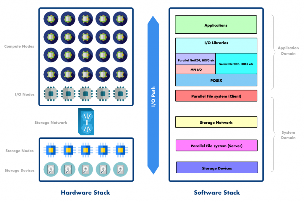
Here is a very high level overview : On the hardware side application is executed on compute nodes. I/O operations issued during the course of an execution are forwarded to I/O nodes which can temporarily store I/O requests and performs some optimization (e.g. I/O aggregation). The I/O nodes then push data through storage network to storage nodes who are responsible for storing data on storage devices. On the software side parallel applications often use MPI I/O or high level I/O libraries like HDF5, NetCDF to map application data into portable, self describing data format. Libraries like HDF5, NetCDF use MPI I/O underneath to benefit from existing I/O optimizations (see this and this). After aggregating I/O operations, parallel filesystem client forwards POSIX request to parallel filesystem server who finally writes application data to a storage device.

To achieve good parallel I/O performance we typically need to:

Perform few I/O operations with large transfer size (transfer should be a multiple of block or stripe size)
Perform collective I/O operations whenever possible
Avoid large number of metadata operations (e.g. independent open/close statements)
Avoid random access i.e. maximise contiguous access
Avoid explicit flushes except when needed for consistency

So what do we want to understand? When application is executing on compute nodes and performing I/O, we want to measure I/O performance and reason about the same. When data flows from application to storage device through various layers (NetCDF, HDF5, MPI I/O and POSIX), we want to understand execution times, I/O sizes, access patters, I/O statistics etc. Also, we want to get insight into I/O transformations performed by intermediate layers (e.g. MPI I/O).

STEP I : Setting Up Darshan

You can download Darshan from project homepage here. There are two software components:

darshan-runtime: This is installed on a compute system where we instrument and run parallel applications.
darshan-util: This is typically installed on system where we analyze performance logs generated by darshan-runtime.

Darshan is already installed on many HPC systems. If you are using any cluster provisioned by HPC centre, before installing from source, check available modules. If you are using Spack, installing Darshan is as simple as:


spack install darshan-runtime
spack install darshan-util

spack install darshan-runtime

spack install darshan-util

Installing Darshan via source tarball is also simple. Assuming you have dependencies installed (MPI and zlib), you can install Darshan as:


wget ftp://ftp.mcs.anl.gov/pub/darshan/releases/darshan-3.1.8.tar.gz
tar -xvzf darshan-3.1.8.tar.gz

# install darshan-runtime
cd darshan-3.1.8/darshan-runtime
./configure  --prefix=$HOME/darshan/runtime --with-mem-align=8 \
             --with-log-path-by-env=DARSHAN_LOG_DIR_PATH \
             --with-jobid-env=NONE CC=mpicc
make -j && make install

# install darshan-util
cd darshan-3.1.8/darshan-util
./configure --prefix=$HOME/darshan/util
make -j && make install

wget ftp://ftp.mcs.anl.gov/pub/darshan/releases/darshan-3.1.8.tar.gz

tar -xvzf darshan-3.1.8.tar.gz

# install darshan-runtime

cd darshan-3.1.8/darshan-runtime

./configure --prefix=$HOME/darshan/runtime --with-mem-align=8 \

--with-log-path-by-env=DARSHAN_LOG_DIR_PATH \

--with-jobid-env=NONE CC=mpicc

make -j && make install

# install darshan-util

cd darshan-3.1.8/darshan-util

./configure --prefix=$HOME/darshan/util

make -j && make install

Here are some additional details for installation:

DARSHAN_LOG_DIR_PATH environment variable indicates the location where Darshan will store measurement log files. You can set this environment variable at runtime.
If you have job scheduler like SLURM or PBS, you should use --with-jobid-env=SLURM_JOBID or --with-jobid-env=PBS_JOBID.
darshan-job-summary.pl tool from darshan-util requires Perl, pdflatex, epstopdf and gnuplot to be installed.

See detailed build instructions for different platforms here.

STEP II : Instrumenting Application

Once Darshan is installed, we are ready to instrument our application. The instrumentation method to use depends on whether we are building statically or dynamically linked executable. On many cluster environments by default we create dynamically linked executable. In this case we can use LD_PRELOAD environment variable to insert instrumentation at run time without modifying application binary. Here are some examples of how we typically launch MPI applications with LD_PRELOD:


# using slurm
srun -n 16 --export=LD_PRELOAD=$HOME/darshan/runtime/lib/libdarshan.so ./app_exe

# using mpi launcher (e.g. Intel MPI)
mpirun -n 16 -env LD_PRELOAD $HOME/darshan/runtime/lib/libdarshan.so ./app_exe

# using cray
aprun -e LD_PRELOAD=$HOME/darshan/runtime/lib/libdarshan.so ./app_exe

# using slurm

srun -n 16 --export=LD_PRELOAD=$HOME/darshan/runtime/lib/libdarshan.so ./app_exe

# using mpi launcher (e.g. Intel MPI)

mpirun -n 16 -env LD_PRELOAD $HOME/darshan/runtime/lib/libdarshan.so ./app_exe

# using cray

aprun -e LD_PRELOAD=$HOME/darshan/runtime/lib/libdarshan.so ./app_exe

One can also use following but might need some precautions (see Miscellaneous Topics section):


LD_PRELOAD=$HOME/darshan/runtime/lib/libdarshan.so srun -n 16 ./app_exe

LD_PRELOAD=$HOME/darshan/runtime/lib/libdarshan.so srun -n 16 ./app_exe

On platforms like Cray, BlueGene the default linking is static. On Cray system compiler option like -dynamic (as opposed to -static) can be used to produce dynamically linked executable. Also, darshan module is often provided with the necessary changes to MPI compiler wrappers. In this case you can load darshan module and compile your application with Cray compiler wrapper as:


module load darshan
CC app.cpp -o app

module load darshan

CC app.cpp -o app

STEP III : Generating and Analysing Darshan Reports

To understand any new profiling tool I typically start with Predictive Performance Analysis technique : start with an example for which you can model performance on paper. Then, compare your predictions with the performance report provided by profiling tool. This way it's easy to get familiar with the tool first time. Lets look at two examples which are small enough to present in their entirety and demonstrate various Darshan features.

Example 1

In this first MPI example each rank is creating 5 different files and writing 1024 bytes block 1024 times (i.e. 1 MB data per file).


#include <iostream>
#include <string>
#include <vector>
#include <mpi.h>

int main(int argc, char *argv[]) {
    int rank;
    int size;

    // mpi initialization
    MPI_Init(&argc, &argv);
    MPI_Comm_rank(MPI_COMM_WORLD, &rank);
    MPI_Comm_size(MPI_COMM_WORLD, &size);

    // i/o parameters
    const size_t num_files = 5;
    const size_t num_writes = 1024;
    const size_t block_size = 1024;

    // buffer to write
    const std::vector<char> data(block_size, 'A');

    for (size_t i = 0; i < num_files; ++i) {

        // generate different file per rank
        std::string filename = "file_";
        filename += std::to_string(rank) + "_" + std::to_string(i);

        // open new file using MPI_COMM_SELF (independent I/O)
        MPI_File fh;
        MPI_File_open(MPI_COMM_SELF, filename.c_str(), MPI_MODE_CREATE | MPI_MODE_WRONLY, MPI_INFO_NULL, &fh);

        // write same buffer num_writes times
        for(size_t j = 0; j < num_writes; j++) {
            MPI_Status status;
            MPI_File_write(fh, &data[0], block_size, MPI_CHAR, &status);
        }

        // close file
        MPI_File_close(&fh);
    }

    MPI_Finalize();
    return 0;
}

#include <iostream>

#include <string>

#include <vector>

#include <mpi.h>

int main(int argc, char *argv[]) {

int rank;

int size;

// mpi initialization

MPI_Init(&argc, &argv);

MPI_Comm_rank(MPI_COMM_WORLD, &rank);

MPI_Comm_size(MPI_COMM_WORLD, &size);

// i/o parameters

const size_t num_files = 5;

const size_t num_writes = 1024;

const size_t block_size = 1024;

// buffer to write

const std::vector<char> data(block_size, 'A');

for (size_t i = 0; i < num_files; ++i) {

// generate different file per rank

std::string filename = "file_";

filename += std::to_string(rank) + "_" + std::to_string(i);

// open new file using MPI_COMM_SELF (independent I/O)

MPI_File fh;

MPI_File_open(MPI_COMM_SELF, filename.c_str(), MPI_MODE_CREATE | MPI_MODE_WRONLY, MPI_INFO_NULL, &fh);

// write same buffer num_writes times

for(size_t j = 0; j < num_writes; j++) {

MPI_Status status;

MPI_File_write(fh, &data[0], block_size, MPI_CHAR, &status);

}

// close file

MPI_File_close(&fh);

}

MPI_Finalize();

return 0;

}

Assuming we run this program with 64 ranks, we expect to see following from an I/O profiling tool:

Total #files opened : 64 x 5 = 320
Total #write operations : 64 x 5 * 1024 = 327680
Total #read operations : 0
Total write size : 64 x 5 x 1024 x 1024 = 335544320 Byte (320 MB)
Write size per opetaion : 1024 Bytes (1 KB)
Avg size per file : 1024 x 1024 = 1 MB
MPI I/O type : Independent i.e. no collective calls are used

Let's now see if we can get same understanding from Darshan. As discussed before, we can compile and instrument this example as follows. We will use LD_PRELOAD because we are building this on standard linux cluster:


mpicxx example1.cpp -o example1

export DARSHAN_LOG_DIR_PATH=$PWD
mpirun -n 64 -env LD_PRELOAD $DARSHAN_HOME/lib/libdarshan.so ./example1

mpicxx example1.cpp -o example1

export DARSHAN_LOG_DIR_PATH=$PWD

mpirun -n 64 -env LD_PRELOAD $DARSHAN_HOME/lib/libdarshan.so ./example1

Once application finishes, Darshan will generate performance log in the same directory:


→ ls -lrt *.darshan
-r-------- 1 kumbhar bbp 53410 Feb 23 19:02 kumbhar_1_id198425_1.darshan

→ ls -lrt *.darshan

-r-------- 1 kumbhar bbp 53410 Feb 23 19:02 kumbhar_1_id198425_1.darshan

Now we can use various tools provided by darshan-util package to analyse measurement log and generate performance reports. The easiest way to start is darshan-job-summary.pl tool that helps to generate pdf summary report of entire execution:


$ darshan-job-summary.pl kumbhar_1_id198425_1.darshan
...
Slowest unique file time: 1.038304
Slowest shared file time: 0
Total bytes read and written by app (may be incorrect): 335544320
Total absolute I/O time: 1.038304
**NOTE: above shared and unique file times calculated using MPI-IO timers if MPI-IO interface used on a given file, POSIX timers otherwise.

$ darshan-job-summary.pl kumbhar_1_id198425_1.darshan

...

Slowest unique file time: 1.038304

Slowest shared file time: 0

Total bytes read and written by app (may be incorrect): 335544320

Total absolute I/O time: 1.038304

**NOTE: above shared and unique file times calculated using MPI-IO timers if MPI-IO interface used on a given file, POSIX timers otherwise.

Above command will generate a pdf file with the same name as performance log file i.e. kumbhar_1_id198425_1.darshan.pdf (see full report in the last section). Let's understand important sections of the report:

example1_1

(1) shows information about the job, number of MPI ranks and runtime of the application.
(2) shows total data transferred and I/O bandwidth observed at MPI layer.
(3) shows amount of time spent in I/O vs. non-IO part of the application. In our example we see that the write operations took very small fraction of the total execution time.
(4) shows that metadata operations are taking long time. Also, time spent in metadata operations at POSIX layer is less compared to MPI layer.
(5) shows write operations are performed using MPI independent I/O i.e. no MPI collective API is used.
(6) shows number of MPI and POSIX operations. In our example POSIX operations count == MPI operations count which indicates that each MPI I/O operation translated into separate POSIX operation.

example1_2

(7) shows histogram of MPI I/O operations and their associated sizes. In our example all I/O operations are of 100-1024 Bytes and in total there are ~32k operations.
(8) shows how MPI I/O operations are translated into low level POSIX I/O operations. In our example POSIX I/O operation size (101-1k) as well total operations count (~32K) are same as MPI. This means each individual MPI operation is translated to equivalent POSIX operation. This behavior is expected considering use of independent MPI I/O.

example1_3

(9) shows most common I/O sizes at MPI and POSIX layer. In our example all accesses were with 1024 bytes and in total there were 327680 operations.
(10) shows how many files were created, how many were read only vs how many were write only and their avg/max sizes. In our example, there were 320 write only files with avg/max size was 1 MB.

example1_4

(11) shows timespan for individual file from the first access to the last access (X-axis is time dimension and Y-axis is MPI rank). We see small dots because each file was accessed for only small duration.
(12) is same as (11) but for shared files. As there are no shared files, this plot is empty.

example1_5

(13) shows the I/O pattern (type of offsets) for each file opened by the application. As our applications writes 1024 bytes to a file without any gaps, offsets were both sequential as well as consecutive. Usually a consecutive pattern is higher performance than an sequential pattern.

If we compare all above statistics, it is clear that the I/O information captured and presented by Darshan is consistent our initial estimates.

Example 2

In the second example we are going to use MPI collective I/O API where each rank is collectively writing 16 blocks of 1024 integers. Each such block is separated by 64 blocks (i.e. 64 x 1024 integers = 262144 bytes). Assuming 64 MPI ranks used in total, the file layout will look like below:

mpi-io-file-layout

The code uses MPI Derived Data type to represent above file view. This example is also small and self explanatory:


#include <iostream>
#include <string>
#include <vector>
#include <mpi.h>

int main(int argc, char *argv[]) {

    int rank;
    int size;

    // mpi initialization
    MPI_Init(&argc, &argv);
    MPI_Comm_rank(MPI_COMM_WORLD, &rank);
    MPI_Comm_size(MPI_COMM_WORLD, &size);

    // i/o parameters
    const int num_files = 5;
    const int num_blocks = 16;
    const int block_size = 1024;

    // buffer to write
    const std::vector<int> data(block_size*num_blocks, rank);

    for(int i = 0; i < num_files; i++) {

        // same filename for all ranks
        std::string filename = "file_";
        filename += std::to_string(i);

        // open new file using MPI_COMM_WORLD (collective I/O)
        MPI_File fh;
        MPI_File_open(MPI_COMM_WORLD, filename.c_str(), MPI_MODE_CREATE | MPI_MODE_WRONLY, MPI_INFO_NULL, &fh);

        // create derived data type
        // 16 blocks, each block of 1024 elements and separated by 64x1024 elements
        MPI_Datatype filetype;
        MPI_Type_vector(num_blocks, block_size, size*block_size, MPI_INT, &filetype);
        MPI_Type_commit(&filetype);

        // calculate offset for each rank and set file view
        MPI_Offset offset = rank * block_size * sizeof(int);
        MPI_File_set_view(fh, offset, MPI_INT, filetype, "native",MPI_INFO_NULL );
        MPI_Type_free(&filetype);

        // write to file collectively
        MPI_Status status;
        MPI_File_write_all(fh, &data[0], block_size*num_blocks, MPI_INT, &status);

        MPI_File_close(&fh);
    }

    MPI_Finalize();
    return 0;
}

#include <iostream>

#include <string>

#include <vector>

#include <mpi.h>

int main(int argc, char *argv[]) {

int rank;

int size;

// mpi initialization

MPI_Init(&argc, &argv);

MPI_Comm_rank(MPI_COMM_WORLD, &rank);

MPI_Comm_size(MPI_COMM_WORLD, &size);

// i/o parameters

const int num_files = 5;

const int num_blocks = 16;

const int block_size = 1024;

// buffer to write

const std::vector<int> data(block_size*num_blocks, rank);

for(int i = 0; i < num_files; i++) {

// same filename for all ranks

std::string filename = "file_";

filename += std::to_string(i);

// open new file using MPI_COMM_WORLD (collective I/O)

MPI_File fh;

MPI_File_open(MPI_COMM_WORLD, filename.c_str(), MPI_MODE_CREATE | MPI_MODE_WRONLY, MPI_INFO_NULL, &fh);

// create derived data type

// 16 blocks, each block of 1024 elements and separated by 64x1024 elements

MPI_Datatype filetype;

MPI_Type_vector(num_blocks, block_size, size*block_size, MPI_INT, &filetype);

MPI_Type_commit(&filetype);

// calculate offset for each rank and set file view

MPI_Offset offset = rank * block_size * sizeof(int);

MPI_File_set_view(fh, offset, MPI_INT, filetype, "native",MPI_INFO_NULL );

MPI_Type_free(&filetype);

// write to file collectively

MPI_Status status;

MPI_File_write_all(fh, &data[0], block_size*num_blocks, MPI_INT, &status);

MPI_File_close(&fh);

}

MPI_Finalize();

return 0;

}

Assuming we run this example with 64 MPI ranks, this is what we expect:

Total #files opened : 5
Total #write operations : 64 x 5 = 320
Total #read operations : 0
Total #write size : 64 x 5 x 1024 x 4 x 16 = 20971520 Bytes (20 MB)
MPI Write size per opetaion : 1024 x 4 x 16 = 65536 Bytes
Avg size per file : 64 x 1024 x 4 x 16 = 4 MB
MPI I/O type : Collective

Similar to Example 1, let's compile and run this application with Darshan instrumentation:


mpicxx example2.cpp -o example2

export DARSHAN_LOG_DIR_PATH=$PWD
mpirun -n 64 -env LD_PRELOAD $DARSHAN_HOME/lib/libdarshan.so ./example2

mpicxx example2.cpp -o example2

export DARSHAN_LOG_DIR_PATH=$PWD

mpirun -n 64 -env LD_PRELOAD $DARSHAN_HOME/lib/libdarshan.so ./example2

Next we have to convert Darshan log into graphical performance report as:


$ darshan-job-summary.pl kumbhar_2_id194151_2.darshan

Slowest shared file time: 1.765187
Total bytes read and written by app (may be incorrect): 20971520
Total absolute I/O time: 1.765187
**NOTE: above shared and unique file times calculated using MPI-IO timers if MPI-IO interface used on a given file, POSIX timers otherwise.

$ darshan-job-summary.pl kumbhar_2_id194151_2.darshan

Slowest shared file time: 1.765187

Total bytes read and written by app (may be incorrect): 20971520

Total absolute I/O time: 1.765187

**NOTE: above shared and unique file times calculated using MPI-IO timers if MPI-IO interface used on a given file, POSIX timers otherwise.

As we have discussed most parts of Darshan report in Example 1, let's focus on important changes:

example2_all

(1) shows huge difference between execution time of MPI I/O write operations and corresponding POSIX operations. This might be because MPI doing extra work before calling POSIX API.
(2) shows MPI collective operations are used for opening file as well as writing.
(3) shows huge different between MPI and POSIX write operations count. This means, large number of MPI operations are combined into few POSIX operations.
(4) shows that 320 MPI I/O operations are reduced to only 5 POSIX write operations i.e. only one write operation per file! If you are familiar with Data Sieving and Collective I/O optimizations then this will be pretty clear.
(5) shows that small MPI I/O operations of few KBs are now combined into MBs size POSIX operations.
(6) shows data from all 64 ranks is collected to one rank to write 4MB file in single POSIX write operation.
(7) shows timespan where all processes are writing to the same shared file. Overall POSIX I/O is taking very small time.

This summarises at large how Darshan can be used for application I/O characterisation.

Command Line Tools

In most of the situations the graphical report generated by darshan-job-summary.pl is sufficient to understand application performance and bottlenecks. But, sometime we need to look at raw performance counters or manipulate darshan logs to zoom into details. There are bunch of command line tools provided by darshan-util package for this purpose. We wouldn't go into details but provide brief summary of different utilities with command line options to give an idea of what is possible:

darshan-convert Converts an existing log file to the newest log format. Also has command line options for anonymizing personal data, adding metadata annotation to the log header, and restricting the output to a specific instrumented file.


$ darshan-convert
Usage: darshan-convert [options] <infile> <outfile>
       Converts darshan log from infile to outfile.
       rewrites the log file into the newest format.
       --bzip2 Use bzip2 compression instead of zlib.
       --obfuscate Obfuscate items in the log.
       --key <key> Key to use when obfuscating.
       --annotate <string> Additional metadata to add.
       --file <hash> Limit output to specified (hashed) file only.
       --reset-md Reset old metadata during conversion.

$ darshan-convert

Usage: darshan-convert [options] <infile> <outfile>

Converts darshan log from infile to outfile.

rewrites the log file into the newest format.

--bzip2 Use bzip2 compression instead of zlib.

--obfuscate Obfuscate items in the log.

--key <key> Key to use when obfuscating.

--annotate <string> Additional metadata to add.

--file <hash> Limit output to specified (hashed) file only.

--reset-md Reset old metadata during conversion.

darshan-parser Utility to obtain a complete, human-readable, text-format dump of all information from Darshan log file.


$ darshan-parser
Usage: darshan-parser [options] <filename>
    --all   : all sub-options are enabled
    --base  : darshan log field data [default]
    --file  : total file counts
    --file-list  : per-file summaries
    --file-list-detailed  : per-file summaries with additional detail
    --perf  : derived perf data
    --total : aggregated darshan field data```

$ darshan-parser

Usage: darshan-parser [options] <filename>

--all : all sub-options are enabled

--base : darshan log field data [default]

--file : total file counts

--file-list : per-file summaries

--file-list-detailed : per-file summaries with additional detail

--perf : derived perf data

--total : aggregated darshan field data```

darshan-summary-per-file.sh Similar to darshan-job-summary.pl except it produces a separate pdf report for every file accessed by an application.


$ darshan-summary-per-file.sh
Usage: darshan-summary-per-file.sh <input_file.darshan> <output_directory>

$ darshan-summary-per-file.sh

Usage: darshan-summary-per-file.sh <input_file.darshan> <output_directory>

darshan-merge Allow per-process logs generated by the mmap-based logging mechanism to be converted into Darshan’s traditional compressed per-job log files.


$ darshan-merge
Usage: darshan-merge --output <output_path> [options] <input_log_glob>
<input_log_glob> is a pattern that matches all input log files (e.g., /log-path/*.darshan).
Options:
    --output    (REQUIRED) Full path of the output darshan log file.
    --shared-redux  Reduce globally shared records into a single record.
    --job-end-time  Set the output log's job end time (requires argument of seconds since Epoch).

$ darshan-merge

Usage: darshan-merge --output <output_path> [options] <input_log_glob>

<input_log_glob> is a pattern that matches all input log files (e.g., /log-path/*.darshan).

Options:

--output (REQUIRED) Full path of the output darshan log file.

--shared-redux Reduce globally shared records into a single record.

--job-end-time Set the output log's job end time (requires argument of seconds since Epoch).

darshan-analyzer Walks an entire directory tree of Darshan log files and produces a summary of the types of access methods used in those log files.


$ darshan-analyzer <directory>

$ darshan-analyzer <directory>

Miscellaneous Topics

Here are some of the important items that I often come across and good to know while using Darshan.

LD_PRELOAD not working with MPI launcher

I have often seen this issue with HPE MPT under SLURM. Use of LD_PRELOAD gives following error:


$ LD_PRELOAD=$HOME/darshan/runtime/lib/libdarshan.so mpiexec ./app
MPT ERROR: PMI2_Init

$ srun -n 16 --export=LD_PRELOAD=$HOME/darshan/runtime/lib/libdarshan.so ./app_exe
MPT ERROR: PMI2_Init

$ LD_PRELOAD=$HOME/darshan/runtime/lib/libdarshan.so mpiexec ./app

MPT ERROR: PMI2_Init

$ srun -n 16 --export=LD_PRELOAD=$HOME/darshan/runtime/lib/libdarshan.so ./app_exe

MPT ERROR: PMI2_Init

The only workaround available today with MPT version <=2.21 is to wrap your executable + LD_PRELOAD under shell script and then use it with mpi launcher. For example:


# create shell script
$ cat new_app.exe

#!/bin/sh
export LD_PRELOAD=$HOME/darshan/runtime/lib/libdarshan.so
./app_exe

# and then launch
$ srun -n 16 ./new_app.exe

# create shell script

$ cat new_app.exe

#!/bin/sh

export LD_PRELOAD=$HOME/darshan/runtime/lib/libdarshan.so

./app_exe

# and then launch

$ srun -n 16 ./new_app.exe

Application opens too many files, but I want to analyse one specific file

Applications often read / write to multiple files and reports generated by darshan-job-summary.pl shows performance summary for all files. We can use darshan-summary-per-file.sh but if application is reading/writing thousands of files, then it will generate one pdf file and will take long time. In this case we can extract record id for each file from Darshan log and then generate summary report for that specific file. Here is how we can achieve this:


# first get file ids
$ darshan-parser --file-list kumbhar_2_id194151_2-23-67820-4406290763854369046_1.darshan
...
#  record_id           file_name                               nprocs slowest   avg
2034758700807672521    /gpfs/some-path-here/darshan-post/file_2 64  0.004060    0.003671
3345894683582565541    /gpfs/some-path-here/darshan-post/file_4 64  0.004024    0.003630
6611969976872978970    /gpfs/some-path-here/darshan-post/file_3 64  0.003964    0.003639
12275450437125689432   /gpfs/some-path-here/darshan-post/file_1 64  0.004324    0.003763
14709127382266971008   /gpfs/some-path-here/darshan-post/file_0 64  0.004885    0.004430

# use record_id of the file that you are intrested
# extracted file_2.darshan file will contain performance record only for file_2
$ darshan-convert --file 2034758700807672521 kumbhar_2_id194151_2-23-67820-4406290763854369046_1.darshan file_2.darshan

# use darshan-job-summary.pl
$ darshan-job-summary.pl file_2.darshan

# first get file ids

$ darshan-parser --file-list kumbhar_2_id194151_2-23-67820-4406290763854369046_1.darshan

...

# record_id file_name nprocs slowest avg

2034758700807672521 /gpfs/some-path-here/darshan-post/file_2 64 0.004060 0.003671

3345894683582565541 /gpfs/some-path-here/darshan-post/file_4 64 0.004024 0.003630

6611969976872978970 /gpfs/some-path-here/darshan-post/file_3 64 0.003964 0.003639

12275450437125689432 /gpfs/some-path-here/darshan-post/file_1 64 0.004324 0.003763

14709127382266971008 /gpfs/some-path-here/darshan-post/file_0 64 0.004885 0.004430

# use record_id of the file that you are intrested

# extracted file_2.darshan file will contain performance record only for file_2

$ darshan-convert --file 2034758700807672521 kumbhar_2_id194151_2-23-67820-4406290763854369046_1.darshan file_2.darshan

# use darshan-job-summary.pl

$ darshan-job-summary.pl file_2.darshan

How can I exclude certain directories?
Sometime it is helpful to exclude certain files from Darshan performance analysis. For example, if application is using Python then we don't want to track every python module that it internally loaded. In some of our simulations we load hundreds of input files during initialization phse which we want to exclude. In this case we can use DARSHAN_EXCLUDE_DIRS env variable with list of directories to exclude:


export DARSHAN_EXCLUDE_DIRS=/your-python-path-dir,/home/kumbhar/input

export DARSHAN_EXCLUDE_DIRS=/your-python-path-dir,/home/kumbhar/input

Note that Darshan by default exclude system directories like /etc, /proc, /usr, /bin. One can set DARSHAN_EXCLUDE_DIRS=none to track everything but this will generate huge Darshan logs.

How can I use Darshan with non-MPI applications?

I haven't used this feature but there is an experimental pre-release of Darshan available here that enables instrumentation of non-MPI workloads. See this announcement.

Hey! I have an issue, what to do?

In addition to this documentation, see existing issues on GitLab here and questions on mailing list here. Otherwise send an email to darshan-users@lists.mcs.anl.gov.

How Darshan summary reports look like?

You can also download darshan logs used for this blog post here. Full pdf summary reports generated by Darshan for above examples are here:
kumbhar_1_id.darshan
kumbhar_2_id.darshan

CREDIT

Thanks to fantastic Darshan developer team from ANL and contributors from NERSC for developing and maintaining this wonderful tool. Especially Phil Carns, Shane Snyder, Kevin Harms, Robert Latham and Glenn K. Lockwood!